はじめに
k-meansを使って、有名なtitanicデータをクラスタリングしてみます。
特徴として、単純なアルゴリズムであることや連続変数を扱いやすいこと、統計的な手法でないこと(正規分布を仮定していたりしないこと)などが挙げられます。
titanicデータをk-meansでクラスタリング!
データ読み込み~クラスタの割り当て
# ライブラリをインポート
import seaborn as sns
import pandas as pd
import numpy as np

import matplotlib.pyplot as plt

from sklearn.cluster import KMeans
from sklearn.preprocessing import StandardScaler

import warnings
warnings.simplefilter(action='ignore', category=FutureWarning)
# Titanicデータセットをロード
titanic_df = sns.load_dataset('titanic')

# 今回使用する列のみ残す。またageには欠損があるので、dropna()を行う
titanic_df = titanic_df[['survived', 'age', 'fare']]
titanic_df = titanic_df.dropna()

# titanic_df.head()
# 特徴量を標準化
features = titanic_df[['age', 'fare']]
scaler = StandardScaler()
features_scaled = scaler.fit_transform(features)
# エルボー法で最適なクラスタ数を探す
sse = []  # 各kにおけるSSE(クラスタ内誤差平方和)を格納するリスト
for k in range(1, 11):
    kmeans = KMeans(n_clusters=k, random_state=123)
    kmeans.fit(features_scaled)
    sse.append(kmeans.inertia_)  # SSE(クラスタ内誤差平方和)をリストに追加

# SSEのプロット
plt.figure(figsize=(6, 4))
plt.plot(range(1, 11), sse, marker='o')
plt.title('Elbow Method')
plt.xlabel('Number of clusters')
plt.ylabel('SSE')
plt.show()

# K-meansクラスタリングを実行して、クラスタラベルを得る
kmeans = KMeans(n_clusters=3, random_state=123) # エルボー法より、k=3とする
clusters = kmeans.fit_predict(features_scaled)

titanic_df['cluster'] = clusters
#titanic_df.head()
#クラスタごとの平均を計算
titanic_df.groupby('cluster').agg('mean')
| cluster | survived | age | fare |
|---|---|---|---|
| 0 | 0.3968 | 21.1366 | 21.6443 |
| 1 | 0.7575 | 31.9672 | 222.8972 |
| 2 | 0.3750 | 45.1208 | 32.7964 |
クラスタごとの平均を計算すると、以下のようなことがわかります
- cluster1の生存率が高い
- cluster1は運賃の平均がcluster0,2に比べて高い
- cluster0,2の生存率はだいたい同じ
結果の可視化
# クラスタと生存状況に基づいて色分け
sns.scatterplot(x='age', y='fare', hue='cluster', data=titanic_df , palette=['red', 'blue', 'green'])

plt.title('K-means Clustering of Titanic Data - All Passengers')
plt.xlabel('Age')
plt.ylabel('Fare')

plt.xlim(0, 85)
plt.ylim(0, 550)

plt.show()

散布図によると、3つの群の特徴は、それぞれ以下の通りです。
- Fare(運賃)の高い群
- Fare(運賃)が低く、Age(年齢)の高い群
- Fare(運賃)が低く、Age(年齢)の低い群
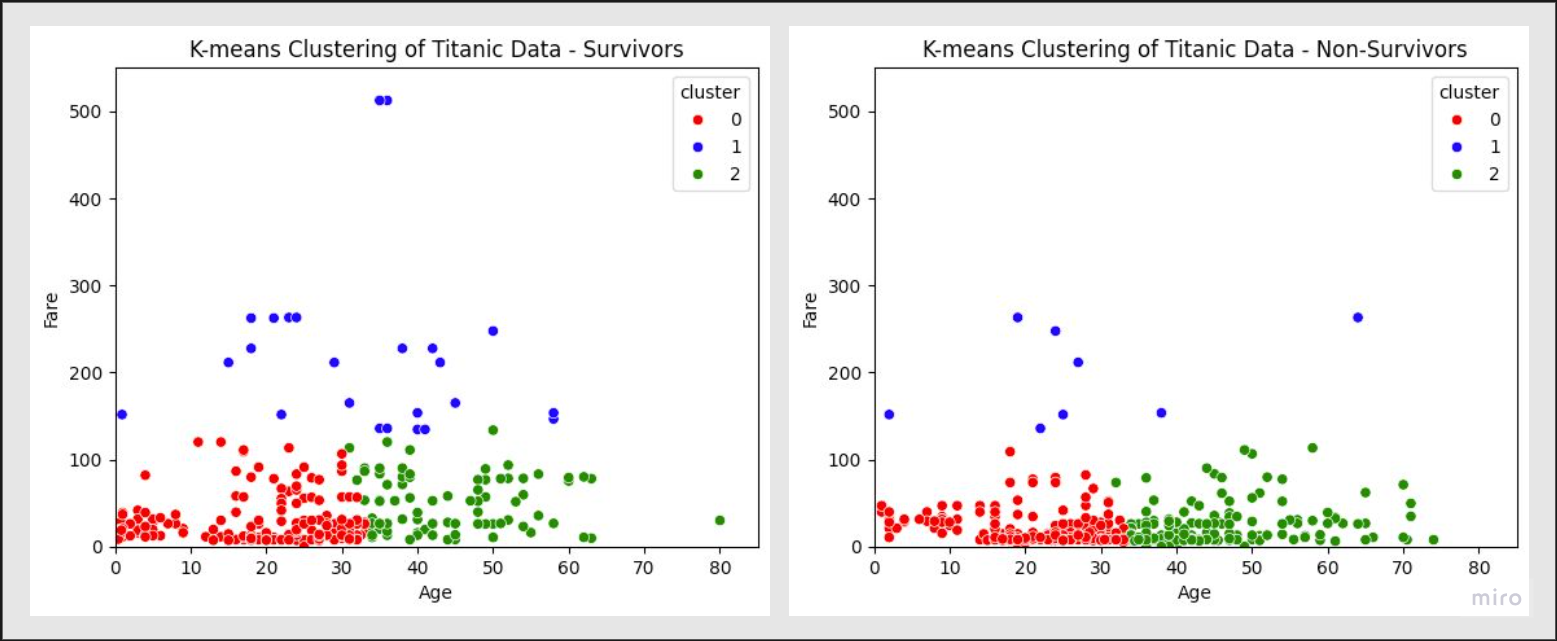
なお、生存群と非生存群とに分けた散布図を下にお示ししています。
これによると、生存群では非生存群に比べてcluster0の0~10歳の点が多いこと、非生存群では生存軍に比べてcluster2の30~50歳の点が多いことが見えてきます。
おわりに
最後までお読みいただきありがとうございました!