【Python】データ分析の序盤でよく使う手法メモ

Kaggleなどでデータ分析を行う際の探索的データ解析（EDA）の段階で、
データの構造を把握する目的で自分自身がよく使う便利な関数やライブラリをまとめました。

データはKaggleのTitanicのTrainデータを使用します
https://www.kaggle.com/c/titanic/data

###■ライブラリの読み込み

import numpy as np
import pandas as pd

###■データの読み込み

df = pd.read_csv('titanic/train.csv')

###■データの基本情報、基本統計量の出力

• まずは最初の5行までを出力し、データを実際に見てみる

df.head()
#()に行数を入力し出力行数を変更可能

• 要約統計量を出力

df.describe()

• オブジェクト型の要素数、ユニーク数、最頻値、最頻 値の出現回数を表示

df.describe(include = 'O')

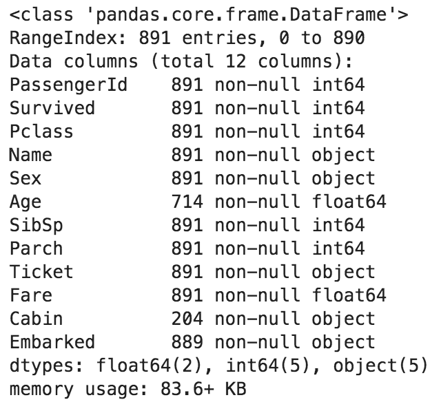
• 全列の（データ数、nullの有無、データ型）を表示

df.info()

• その他便利なコマンド

df.tail() #最後から5行表示
df.shape #(行数, 列数)を表示
df.size #データ数を表示
df.dtypes #データ型を表示
df.columns #列一覧を表示
df.corr() #全列の相関係数表示

###■pandas-profilingでプロファイリング

2行のコードで、読み込むデータの様々な情報をグラフを含めて出力できます

import pandas_profiling #インポート
pandas_profiling.ProfileReport(df) #実行

別記事で詳しく解説しています
https://qiita.com/ryo111/items/705347799a984acd5d08

###■各列のユニーク値の種類数を表示

df.apply(lambda x: x.nunique())

###■各列の欠損値の確認

df.isnull().sum()

###■指定の列の他の列との相関係数を表示

目的変数を入力すれば、他の変数との相関関係をシンプルに出力できるので便利

df.corr()["Survived"].sort_values()

###■数値データ（もしくはオブジェクトデータ）の列のみのインデックスを出力

#数値データのみ
df.select_dtypes(include=[np.number]).columns

#オブジェクトデータのみ
df.select_dtypes(include=[np.object]).columns

###■指定したオブジェクトデータ列の項目を表示

df["Embarked"].unique()

###■指定したオブジェクトデータ列の項目別の数量を表示

df['Embarked'].value_counts()

###■グループバイによる集計

• 性別('Sex')ごとに各変数の平均値(mean)を出力

df.groupby('Sex').mean()

###■ピボットによる集計

• 性別('Sex')をインデックス、乗船場所('Embarked')をカラムとした、生存者('Survived')の合計(sum)の表を出力

df.pivot_table(values='Survived', index='Sex', columns='Embarked', aggfunc='sum')

通常の分析では、ここからさらにグラフを活用しデータの構造をビジュアルで把握していきます。
その際の手法は下記リンク先の別記事でまとめておりますのでご覧ください。
https://qiita.com/ryo111/items/bf24c8cf508ad90cfe2e

その他、欠損値処理のまとめ記事もよろしければご覧ください。
https://qiita.com/ryo111/items/4177c732cc9801bccb17