scikit-learnのデータセットfetch_lfw_people

何これえ
まずはimport

from sklearn.datasets import fetch_lfw_people

import numpy as np
%matplotlib inline
import matplotlib.pyplot as plt

早速ヘルプを見る

help(fetch_lfw_people)

fetch_lfw_people(*, data_home=None, funneled=True, resize=0.5, min_faces_per_person=0, color=False, slice_=(slice(70, 195, None), slice(78, 172, None)), download_if_missing=True, return_X_y=False)

引数を大雑把に説明
resizeは各顔写真の比率で元のデータからの比率となるらしい。defaultは0.5
min_faces_per_personは同一人物の写真が最低何枚あるデータを残すか指定する引数。
後からも見るがこのデータセットには1、2枚しか画像がない人物の写真が大量にある。十分枚数のある画像データだけ残すために使う引数である。
colorはbool値を引数にとり、RGB形式で色を残すかどうかを決める、デフォルトではFalse
デフォルトだと明暗のみが残るといった感じ

他の引数は
return_X_yはbool値をとる。Trueだと.data属性と.target属性のtupleのみ返すようになる。デフォルトはFalse
残りは画像データのダウンロードに関する引数

返り値

dataset : :class:~sklearn.utils.Bunch
Dictionary-like object, with the following attributes.

    data : numpy array of shape (13233, 2914)
        Each row corresponds to a ravelled face image
        of original size 62 x 47 pixels.
        Changing the ``slice_`` or resize parameters will change the
        shape of the output.
    images : numpy array of shape (13233, 62, 47)
        Each row is a face image corresponding to one of the 5749 people in
        the dataset. Changing the ``slice_``
        or resize parameters will change the shape of the output.
    target : numpy array of shape (13233,)
        Labels associated to each face image.
        Those labels range from 0-5748 and correspond to the person IDs.
    DESCR : str
        Description of the Labeled Faces in the Wild (LFW) dataset.

なにも引数をいじらない場合13233枚の画像データが返ってくる。62 x 47 = 2914でわかるとおり、images属性を平坦化したものがdata属性である。

people = fetch_lfw_people()
people_images = []
for arr in people.images:
    people_images.append(arr.ravel())
people_images = np.array(people_images)
np.all(people_images == people.data)

#実行結果
#True

target属性には各画像のラベルが数字で割り当てられている。

np.unique(people.target)

#実行結果
#array([   0,    1,    2, ..., 5746, 5747, 5748])

従って5749名の画像データがあることがわかる。
ただ、一人一人の画像数は全く均等ではない

np.min(np.bincount(people.target))
#実行結果
#1

np.max(np.bincount(people.target))
#実行結果
#530

画像を一枚しか持たない持たない人もいれば、530枚持っている人もいる。

plt.figure(figsize=(12, 8))
plt.hist(np.bincount(people.target), bins=np.arange(1, 531))
plt.yscale("log");

上のグラフはx軸が画像を持っている枚数でy軸がその枚数持っている人数の合計である。
１、2枚程度しか画像を持っていない人物が非常に多いわけである。

DESCR属性にはこのデータセットの情報が書いてある。
http://vis-www.cs.umass.edu/lfw/

最初の10枚のデータを表示する

fig, axes = plt.subplots(2, 5, figsize=(9, 3),
                         subplot_kw={"xticks": (), "yticks": ()})
for ax, image, name in zip(axes.ravel(), people.images, people.target):
    ax.imshow(image)
    ax.set_title(people.target_names[name].split()[-1])
fig.tight_layout()

plt.imshow()　の詳細

ちなみにplt.imshow()は配列を解釈して色をつけて返す関数

fig, axes = plt.subplots(1, 4, figsize=(16, 4))

arr = np.arange(25).reshape(5, 5)
axes[0].imshow(arr)

arr1 = arr * 10
axes[1].imshow(arr1)

arr2 = arr / arr.max()
axes[2].imshow(arr2)

arr3 = arr + 1000
axes[3].imshow(arr3);

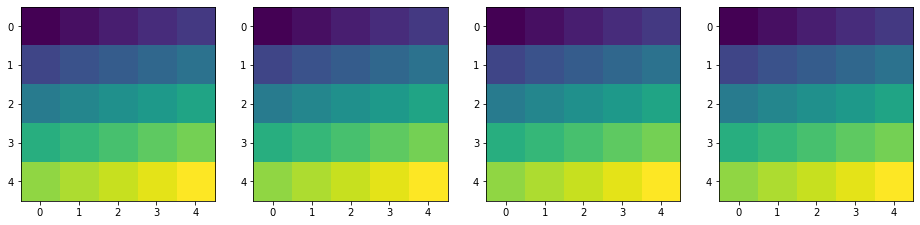
このように表示される画像は全部同じになっているのがわかる。配列の各要素の差の幅で明暗を決めているっぽい。

主成分分析してみる

主成分分析とは？
私には分からん

from sklearn.decomposition import PCA
pca = PCA.fit(people.data)
fig, axes = plt.subplots(4, 5, figsize=(10, 8),
            subplot_kw={"xticks": (), "yticks": ()})
for component, ax in zip(pca.components_, axes.ravel()):
    ax.imshow(component.reshape(image_shape))

主成分分析は分散が大きい方向から順番に主成分を取り出す。
今回は100番目まで取り出している。表示しているのは最初の20番目

画像の再構成

inverse_transformメソッドを使えば、主成分の重ね合わせから画像を再構成できるようなので、やってみる。

from sklearn.decomposition import PCA
from sklearn.datasets import fetch_lfw_people
people = fetch_lfw_people()
X = people.data
y = people.target
pca = PCA(n_components=100, random_state=0)
X_pca = pca.fit_transform(X)
image_shape = people.images[0].shape
X_pca_inverse = pca.inverse_transform(X_pca)
fig, axes = plt.subplots(4, 5, figsize=(10, 8),
                         subplot_kw={"xticks": (), "yticks": ()})
for ax, data, target in zip(axes.ravel(), X_pca_inverse, y):
    ax.imshow(data.reshape(image_shape))
    ax.set_title(people.target_names[target].split()[-1])

ちなみに元の画像

次元を100に落としたので、メガネとかひげとかはぶん取られてしまった。

まとめ

fetch_lfw_people は有名人の顔写真をまとめたデータセットである。
一人当たりの画像数にはだいぶばらつきがある。
アメリカ人がほとんど（だと思う）
ブッシュ大統領の写真が530枚と圧倒的に多い。
取り扱うときには画像が少なすぎる人を弾いたり、画像が多すぎる人の枚数を減らしたりした方がいいかもしれない。