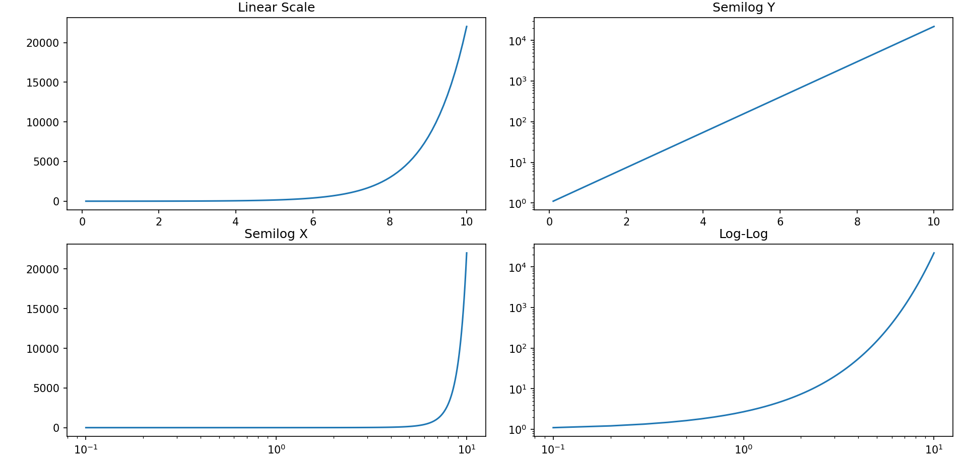
片対数グラフ、両対数グラフ
import matplotlib.pyplot as plt
import numpy as np

# サンプルデータ生成
x = np.linspace(0.1, 10, 100)
y = np.exp(x)  # 例として指数関数を使用

# プロット
fig, axs = plt.subplots(2, 2, figsize=(10, 8))

# 線形スケール
axs[0, 0].plot(x, y)
axs[0, 0].set_title('Linear Scale')

# 片対数スケール
axs[0, 1].plot(x, y)
axs[0, 1].set_yscale('log')
axs[0, 1].set_title('Semilog Y')

# 片対数スケール (x)
axs[1, 0].plot(x, y)
axs[1, 0].set_xscale('log')
axs[1, 0].set_title('Semilog X')

# 両対数スケール
axs[1, 1].plot(x, y)
axs[1, 1].set_xscale('log')
axs[1, 1].set_yscale('log')
axs[1, 1].set_title('Log-Log')

plt.tight_layout()
plt.show()
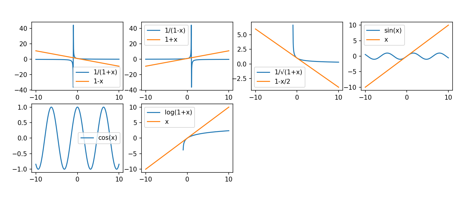
テイラー展開と線形近似
import numpy as np
import matplotlib.pyplot as plt

# 関数の定義
def func1(x):
    return 1 / (1 + x)

def func2(x):
    return 1 - x

def func3(x):
    return 1 / (1 - x)

def func4(x):
    return 1 + x

def func5(x):
    return 1 / np.sqrt(1 + x)

def func6(x):
    return 1 - x / 2

def func7(x):
    return np.sin(x)

def func8(x):
    return x

def func9(x):
    return np.cos(x)

def func10(x):
    return 1

def func11(x):
    return np.log(1 + x)

def func12(x):
    return x

# xの範囲を設定
x = np.linspace(-10, 10, 400)

# 関数の評価
y1 = func1(x)
y2 = func2(x)
y3 = func3(x)
y4 = func4(x)
y5 = func5(x)
y6 = func6(x)
y7 = func7(x)
y8 = func8(x)
y9 = func9(x)
y10 = func10(x)
y11 = func11(x)
y12 = func12(x)

# グラフの描画
plt.figure(figsize=(12, 8))

# 関数1と2のグラフ
plt.subplot(3, 4, 1)
plt.plot(x, y1, label='1/(1+x)')
plt.plot(x, y2, label='1-x')
plt.legend()

# 関数3と4のグラフ
plt.subplot(3, 4, 2)
plt.plot(x, y3, label='1/(1-x)')
plt.plot(x, y4, label='1+x')
plt.legend()

# 関数5と6のグラフ
plt.subplot(3, 4, 3)
plt.plot(x, y5, label='1/√(1+x)')
plt.plot(x, y6, label='1-x/2')
plt.legend()

# 関数7と8のグラフ
plt.subplot(3, 4, 4)
plt.plot(x, y7, label='sin(x)')
plt.plot(x, y8, label='x')
plt.legend()

# 関数9と10のグラフ
plt.subplot(3, 4, 5)
plt.plot(x, y9, label='cos(x)')
plt.plot(x, y10, label='1')
plt.legend()

# 関数11と12のグラフ
plt.subplot(3, 4, 6)
plt.plot(x, y11, label='log(1+x)')
plt.plot(x, y12, label='x')
plt.legend()

plt.show()
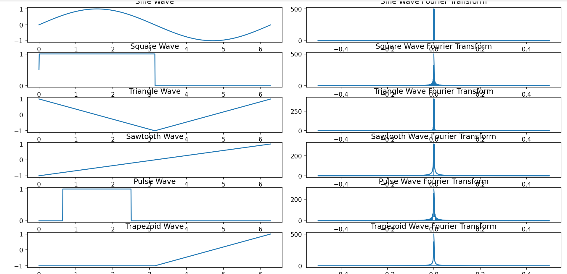
# プロット
plt.figure(figsize=(12, 16))

# 正弦波の入力波形
plt.subplot(6, 2, 1)
x = np.linspace(0, period, num_samples, endpoint=False)
plt.plot(x, sine_wave(x))
plt.title('Sine Wave')

# 正弦波のフーリエ変換
plt.subplot(6, 2, 2)
plt.plot(sine_freqs, sine_fourier)
plt.title('Sine Wave Fourier Transform')

# 正方波の入力波形
plt.subplot(6, 2, 3)
plt.plot(x, square_wave(x))
plt.title('Square Wave')

# 正方波のフーリエ変換
plt.subplot(6, 2, 4)
plt.plot(square_freqs, square_fourier)
plt.title('Square Wave Fourier Transform')

# 三角波の入力波形
plt.subplot(6, 2, 5)
plt.plot(x, triangle_wave(x))
plt.title('Triangle Wave')

# 三角波のフーリエ変換
plt.subplot(6, 2, 6)
plt.plot(triangle_freqs, triangle_fourier)
plt.title('Triangle Wave Fourier Transform')

# のこぎり波の入力波形
plt.subplot(6, 2, 7)
plt.plot(x, sawtooth_wave(x))
plt.title('Sawtooth Wave')

# のこぎり波のフーリエ変換
plt.subplot(6, 2, 8)
plt.plot(sawtooth_freqs, sawtooth_fourier)
plt.title('Sawtooth Wave Fourier Transform')

# パルス波の入力波形
plt.subplot(6, 2, 9)
plt.plot(x, pulse_wave(x))
plt.title('Pulse Wave')

# パルス波のフーリエ変換
plt.subplot(6, 2, 10)
plt.plot(pulse_freqs, pulse_fourier)
plt.title('Pulse Wave Fourier Transform')

# 台形波の入力波形
plt.subplot(6, 2, 11)
plt.plot(x, trapezoid_wave(x))
plt.title('Trapezoid Wave')

# 台形波のフーリエ変換
plt.subplot(6, 2, 12)
plt.plot(trapezoid_freqs, trapezoid_fourier)
plt.title('Trapezoid Wave Fourier Transform')

plt.tight_layout()
plt.show()
波形が崩れてしまった
ラプラス変換
2階微分方程式と伝達関数について
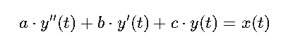
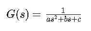
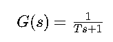
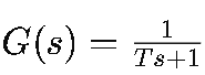
伝達関数
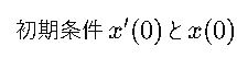
1,y(t)をラプラス変換してY(s)とする
2.初期条件((as+b)x(0)+ax'(0))を求める
3,Y(s)×伝達関数G(s)+ ((as+b)x(0)+ax'(0))×伝達関数G(s)=X(s)
4,X(s)を逆ラプラス変換してx(t)を求める
ラプラス変換計算ツール
https://blog.yfsakai.com/posts/2016-09-18-wolframalpha-how-to-laplace-inverse-laplace/
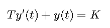
Kはゲイン
Tは時定数
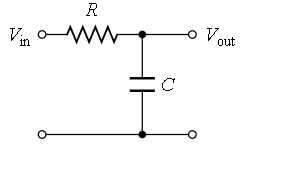
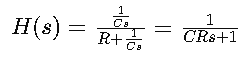
例 ローパスフィルタ
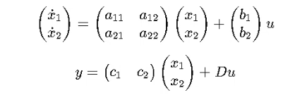
微分方程式で表された状態方程式