PWM変調のプログラム

import numpy as np
import matplotlib.pyplot as plt

# PWM parameters
frequency = 50  # Hz
period = 1 / frequency  # seconds
sampling_rate = 10000  # samples per second
t = np.linspace(0, 2 * period, int(sampling_rate * 2 * period), endpoint=False)  # Time array

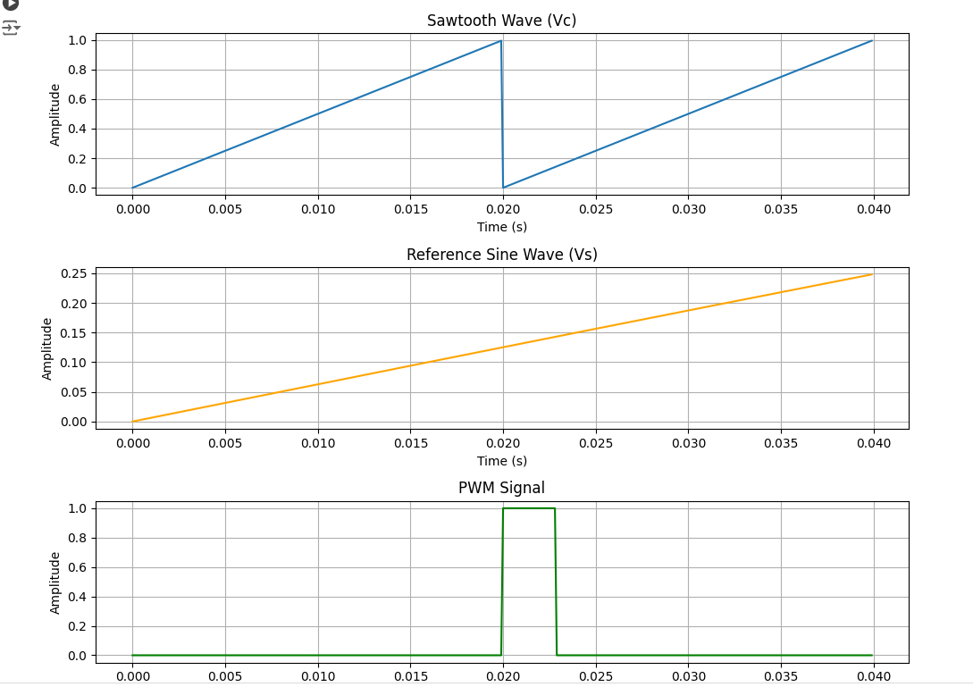
# Create a sawtooth wave (carrier signal)
Vc = np.mod(t, period) / period

# Define the reference sine wave (Vs)
Vs_frequency = 1  # Hz
Vs_amplitude = 1
Vs = Vs_amplitude * np.sin(2 * np.pi * Vs_frequency * t)

# Generate the PWM signal
PWM_signal = np.where(Vs > Vc, 1, 0)

# Plotting
plt.figure(figsize=(10, 8))

# Plot the carrier signal (sawtooth wave)
plt.subplot(3, 1, 1)
plt.plot(t, Vc, label='Sawtooth Wave (Vc)')
plt.title('Sawtooth Wave (Vc)')
plt.xlabel('Time (s)')
plt.ylabel('Amplitude')
plt.grid(True)

# Plot the reference signal (sine wave)
plt.subplot(3, 1, 2)
plt.plot(t, Vs, label='Reference Sine Wave (Vs)', color='orange')
plt.title('Reference Sine Wave (Vs)')
plt.xlabel('Time (s)')
plt.ylabel('Amplitude')
plt.grid(True)

# Plot the PWM signal
plt.subplot(3, 1, 3)
plt.plot(t, PWM_signal, label='PWM Signal', color='green')
plt.title('PWM Signal')
plt.xlabel('Time (s)')
plt.ylabel('Amplitude')
plt.grid(True)

plt.tight_layout()
plt.show()

import numpy as np
import matplotlib.pyplot as plt

# PWM parameters
frequency = 5000  # Hz for the triangular wave
period = 1 / frequency  # seconds
sampling_rate = 10000000  # samples per second
t = np.linspace(0, 2 * period, int(sampling_rate * 2 * period), endpoint=False)  # Time array

# Create a triangular wave (input B)
B = 2 * np.abs(2 * (t / period - np.floor(t / period + 0.5))) - 1

# Define the reference sine wave (input A)
A_frequency = 1  # Hz
A_amplitude = 1
A = A_amplitude * np.sin(2 * np.pi * A_frequency * t)

# Generate the comparator output (input C)
C = np.where(A > B, 1, 0)

# Define RL circuit parameters
R = 1  # ohms
L = 0.01  # henries
V_dc = 5  # DC voltage in volts

# Initialize current array for the RL circuit
I = np.zeros_like(t)
dt = t[1] - t[0]  # Time step

# Simulate the RL circuit
for i in range(1, len(t)):
    dI_dt = (V_dc * C[i-1] - R * I[i-1]) / L
    I[i] = I[i-1] + dI_dt * dt

# Plotting
plt.figure(figsize=(12, 10))

# Plot the sine wave (input A)
plt.subplot(4, 1, 1)
plt.plot(t, A, label='Sine Wave (Input A)')
plt.title('Sine Wave (Input A)')
plt.xlabel('Time (s)')
plt.ylabel('Amplitude')
plt.grid(True)

# Plot the triangular wave (input B)
plt.subplot(4, 1, 2)
plt.plot(t, B, label='Triangular Wave (Input B)', color='orange')
plt.title('Triangular Wave (Input B)')
plt.xlabel('Time (s)')
plt.ylabel('Amplitude')
plt.grid(True)

# Plot the comparator output (input C)
plt.subplot(4, 1, 3)
plt.plot(t, C, label='Comparator Output (Input C)', color='green')
plt.title('Comparator Output (Input C)')
plt.xlabel('Time (s)')
plt.ylabel('Amplitude')
plt.grid(True)

# Plot the RL circuit current
plt.subplot(4, 1, 4)
plt.plot(t, I, label='Current through RL Circuit', color='red')
plt.title('Current through RL Circuit')
plt.xlabel('Time (s)')
plt.ylabel('Current (A)')
plt.grid(True)

plt.tight_layout()
plt.show()

import numpy as np
import matplotlib.pyplot as plt

# 搬送波（三角波）の生成
f_carrier = 1000  # 搬送波の周波数 [Hz]
t = np.linspace(0, 0.01, num=1000)  # 時間配列 [s]
carrier_wave = 0.5 * (1 + np.sin(2 * np.pi * f_carrier * t))

# 基本波（正弦波）の生成
f_signal = 50  # 基本波の周波数 [Hz]
signal_wave = np.sin(2 * np.pi * f_signal * t)

# PWM制御による出力信号の生成
pwm_output = np.zeros_like(t)
for i in range(len(t)):
    if signal_wave[i] > carrier_wave[i]:
        pwm_output[i] = 1
    else:
        pwm_output[i] = 0

# プロット設定
plt.figure(figsize=(10, 6))

plt.subplot(3, 1, 1)
plt.plot(t, carrier_wave, label='Carrier Wave (Triangle)')
plt.ylabel('Amplitude')
plt.legend()

plt.subplot(3, 1, 2)
plt.plot(t, signal_wave, label='Signal Wave (Sine)')
plt.ylabel('Amplitude')
plt.legend()

plt.subplot(3, 1, 3)
plt.step(t, pwm_output, where='mid', label='PWM Output')
plt.ylabel('Output')
plt.xlabel('Time [s]')
plt.ylim([-0.1, 1.1])
plt.legend()

plt.tight_layout()
plt.show()

他の変調

import numpy as np
import matplotlib.pyplot as plt

# 基本パラメータ
fs = 1000  # サンプリング周波数
t = np.arange(0, 1, 1/fs)  # 時間ベクトル
f_carrier = 50  # 搬送波周波数
f_signal = 5    # 変調信号周波数
amplitude = 1   # 振幅

# 変調信号（正弦波）
modulating_signal = np.sin(2 * np.pi * f_signal * t)

# 振幅変調（AM）
am_signal = (1 + modulating_signal) * np.cos(2 * np.pi * f_carrier * t)

# 周波数変調（FM）
kf = 10  # 周波数感度
fm_signal = np.cos(2 * np.pi * f_carrier * t + kf * np.cumsum(modulating_signal) / fs)

# 位相変調（PM）
kp = np.pi / 2  # 位相感度
pm_signal = np.cos(2 * np.pi * f_carrier * t + kp * modulating_signal)

# プロット
plt.figure(figsize=(12, 8))

# 振幅変調
plt.subplot(3, 1, 1)
plt.plot(t, am_signal)
plt.title('Amplitude Modulation (AM)')
plt.xlabel('Time [s]')
plt.ylabel('Amplitude')

# 周波数変調
plt.subplot(3, 1, 2)
plt.plot(t, fm_signal)
plt.title('Frequency Modulation (FM)')
plt.xlabel('Time [s]')
plt.ylabel('Amplitude')

# 位相変調
plt.subplot(3, 1, 3)
plt.plot(t, pm_signal)
plt.title('Phase Modulation (PM)')
plt.xlabel('Time [s]')
plt.ylabel('Amplitude')

plt.tight_layout()
plt.show()

import numpy as np
import matplotlib.pyplot as plt

# Define time array
t = np.linspace(0, 0.01, 10000)  # 10ms duration, high resolution

# Define the modulating wave (A) - a sinusoidal wave with frequency 50Hz
freq_modulating = 50  # in Hz
modulating_wave = np.sin(2 * np.pi * freq_modulating * t)

# Define the carrier wave (B) - a triangle wave with frequency 50kHz
freq_carrier = 5000  # in Hz
carrier_wave = np.abs(2 * (t * freq_carrier - np.floor(0.5 + t * freq_carrier)))

# Comparator output: 1 if modulating wave > carrier wave, else 0
comparator_output = np.where(modulating_wave > carrier_wave, 1, 0)

# Plot the modulating wave (A)
plt.figure(figsize=(15, 6))

plt.subplot(3, 1, 1)
plt.plot(t, modulating_wave, label='Modulating Wave (50Hz)')
plt.title('Modulating Wave ')
plt.xlabel('Time [s]')
plt.ylabel('Amplitude')
plt.grid(True)
plt.legend()

# Plot the carrier wave (B)
plt.subplot(3, 1, 2)
plt.plot(t, carrier_wave, label='Carrier Wave (50kHz Triangle)', color='orange')
plt.title('Carrier Wave ')
plt.xlabel('Time [s]')
plt.ylabel('Amplitude')
plt.grid(True)
plt.legend()

# Plot the comparator output
plt.subplot(3, 1, 3)
plt.plot(t, comparator_output, label='Comparator Output', color='green')
plt.title('Comparator Output')
plt.xlabel('Time [s]')
plt.ylabel('Output')
plt.grid(True)
plt.legend()

plt.tight_layout()
plt.show()

import numpy as np
import matplotlib.pyplot as plt

def generate_pwm(frequency, duty_cycle, duration, sampling_rate):
    """
    Generate a PWM signal.

    :param frequency: Frequency of the PWM signal in Hz
    :param duty_cycle: Duty cycle of the PWM signal (0 to 1)
    :param duration: Duration of the signal in seconds
    :param sampling_rate: Sampling rate in Hz
    :return: Time array and PWM signal array
    """
    t = np.arange(0, duration, 1/sampling_rate)
    pwm_signal = ((t * frequency) % 1) < duty_cycle
    return t, pwm_signal.astype(float)

# Parameters
frequency = 10  # PWM frequency in Hz
duty_cycle = 0.9  # Duty cycle (0 to 1)
duration = 1  # Signal duration in seconds
sampling_rate = 1000  # Sampling rate in Hz

# Generate PWM signal
time, pwm_signal = generate_pwm(frequency, duty_cycle, duration, sampling_rate)

# Plot the PWM signal
plt.figure(figsize=(10, 4))
plt.plot(time, pwm_signal)
plt.title(f'PWM Signal - Frequency: {frequency} Hz, Duty Cycle: {duty_cycle * 100}%')
plt.xlabel('Time [s]')
plt.ylabel('Amplitude')
plt.ylim(-0.1, 1.1)
plt.grid()
plt.show()

import numpy as np
import matplotlib.pyplot as plt
from scipy.signal import butter, lfilter

def generate_pwm(frequency, duty_cycle, duration, sampling_rate):
    t = np.arange(0, duration, 1/sampling_rate)
    pwm_signal = ((t * frequency) % 1) < duty_cycle
    return t, pwm_signal.astype(float)

def butter_lowpass_filter(data, cutoff, fs, order=5):
    nyquist = 0.5 * fs
    normal_cutoff = cutoff / nyquist
    b, a = butter(order, normal_cutoff, btype='low', analog=False)
    y = lfilter(b, a, data)
    return y

# Parameters
frequency = 10  # PWM frequency in Hz
duty_cycle = 0.6  # Duty cycle (0 to 1)
duration = 2  # Signal duration in seconds
sampling_rate = 1000  # Sampling rate in Hz
cutoff_frequency = 5  # Low-pass filter cutoff frequency in Hz

# Generate PWM signal
time, pwm_signal = generate_pwm(frequency, duty_cycle, duration, sampling_rate)

# Apply low-pass filter to simulate transient response
filtered_signal = butter_lowpass_filter(pwm_signal, cutoff_frequency, sampling_rate)

# Plot the PWM signal and the filtered signal
plt.figure(figsize=(12, 8))

plt.subplot(3, 1, 1)
plt.plot(time, pwm_signal)
plt.title('PWM Signal')
plt.xlabel('Time [s]')
plt.ylabel('Amplitude')
plt.ylim(-0.1, 1.1)
plt.grid()

plt.subplot(3, 1, 2)
plt.plot(time, pwm_signal, label='Original Transient Response', color='orange')
plt.title('PWM Signal (Zoomed)')
plt.xlabel('Time [s]')
plt.ylabel('Amplitude')
plt.xlim(0, 0.1)  # Zoom in to see the transient behavior
plt.ylim(-0.1, 1.1)
plt.grid()

plt.subplot(3, 1, 3)
plt.plot(time, filtered_signal, label='Filtered Signal', color='green')
plt.title('Filtered Signal (Low-pass Filter)')
plt.xlabel('Time [s]')
plt.ylabel('Amplitude')
plt.ylim(-0.1, 1.1)
plt.grid()

plt.tight_layout()
plt.show()