import sympy as sp

# シンボリック変数の定義
t, s = sp.symbols('t s')
a, b, c, d = sp.symbols('a b c d')
A = sp.Matrix([[a, b], [c, d]])
I = sp.eye(2)

# ラプラス変換を用いた状態遷移行列の計算
Phi_s_laplace = (s * I - A).inv()
Phi_t_laplace = sp.inverse_laplace_transform(Phi_s_laplace, s, t)

# 対角化を用いた状態遷移行列の計算
P, D = A.diagonalize()
Phi_t_diag = P * sp.exp(D * t) * P.inv()

# 結果の表示
print("ラプラス変換を用いた状態遷移行列:")
sp.pprint(Phi_t_laplace)

print("\n対角化を用いた状態遷移行列:")
sp.pprint(Phi_t_diag)
import numpy as np
import scipy.linalg
import matplotlib.pyplot as plt

# システムパラメータの設定
m = 0.2    # 振子の質量 (kg)
M = 0.5    # カートの質量 (kg)
L = 0.3    # 振子の長さ (m)
g = 9.81   # 重力加速度 (m/s^2)
d = 0.1    # 摩擦係数

# 状態空間モデルの行列
A = np.array([[0, 1, 0, 0],
              [0, -d/M, m*g/M, 0],
              [0, 0, 0, 1],
              [0, -d/(M*L), (M+m)*g/(M*L), 0]])

B = np.array([[0],
              [1/M],
              [0],
              [1/(M*L)]])

C = np.array([[1, 0, 0, 0],
              [0, 0, 1, 0]])

D = np.array([[0],
              [0]])

# LQRの重み行列
Q = np.diag([10, 1, 10, 1])
R = np.array([[0.1]])

# リカッチ方程式を解いてLQRゲインを計算
X = np.matrix(scipy.linalg.solve_continuous_are(A, B, Q, R))
K = np.matrix(scipy.linalg.inv(R) * (B.T * X))

# シミュレーションの設定
dt = 0.01  # 時間ステップ (s)
T = 10.0   # シミュレーション時間 (s)
t = np.arange(0, T, dt)

# 初期状態
x = np.array([[0.1],  # 初期カート位置 (m)
              [0.0],  # 初期カート速度 (m/s)
              [0.1],  # 初期振子角度 (rad)
              [0.0]]) # 初期振子角速度 (rad/s)

# シミュレーションの実行
x_history = []
for _ in t:
    u = -K * x  # 制御入力
    x_dot = A * x + B * u  # 状態の微分
    x = x + x_dot * dt  # 状態の更新
    x_history.append(x.A1)  # 状態履歴の保存

x_history = np.array(x_history)

# 結果のプロット
plt.figure(figsize=(10, 8))

plt.subplot(4, 1, 1)
plt.plot(t, x_history[:, 0])
plt.ylabel('Cart Position (m)')
plt.grid(True)

plt.subplot(4, 1, 2)
plt.plot(t, x_history[:, 1])
plt.ylabel('Cart Velocity (m/s)')
plt.grid(True)

plt.subplot(4, 1, 3)
plt.plot(t, x_history[:, 2])
plt.ylabel('Pendulum Angle (rad)')
plt.grid(True)

plt.subplot(4, 1, 4)
plt.plot(t, x_history[:, 3])
plt.ylabel('Pendulum Angular Velocity (rad/s)')
plt.xlabel('Time (s)')
plt.grid(True)

plt.tight_layout()
plt.show()
import numpy as np
import matplotlib.pyplot as plt
from scipy.signal import place_poles, StateSpace, lti, step, lsim

# Define the first-order lag system
a = 1.0  # Time constant
b = 1.0  # Gain

# State-space representation
A = np.array([[-a]])
B = np.array([[b]])
C = np.array([[1.0]])
D = np.array([[0.0]])

print("State-space representation:")
print("A =", A)
print("B =", B)
print("C =", C)
print("D =", D)

# Define observer pole
observer_pole = -5.0  # Desired observer pole

# Calculate observer gain L
L = place_poles(A.T, C.T, [observer_pole]).gain_matrix.T
print("Observer gain L =", L)

# Observer system matrices
A_obs = A - L @ C
B_obs = np.hstack([B, L])
C_obs = C
D_obs = np.zeros((C.shape[0], B_obs.shape[1]))  # Adjusting the shape of D_obs

print("Observer system matrices:")
print("A_obs =", A_obs)
print("B_obs =", B_obs)
print("C_obs =", C_obs)
print("D_obs =", D_obs)

# Calculate the poles of the observer system
observer_poles = np.linalg.eigvals(A_obs)
print("Observer poles =", observer_poles)

# Check controllability
controllability_matrix = np.hstack([B, A @ B])
rank_controllability = np.linalg.matrix_rank(controllability_matrix)
print("Controllability matrix =", controllability_matrix)
print("Rank of controllability matrix =", rank_controllability)
if rank_controllability == A.shape[0]:
    print("The system is controllable.")
else:
    print("The system is not controllable.")

# Check observability
observability_matrix = np.vstack([C, C @ A])
rank_observability = np.linalg.matrix_rank(observability_matrix)
print("Observability matrix =", observability_matrix)
print("Rank of observability matrix =", rank_observability)
if rank_observability == A.shape[0]:
    print("The system is observable.")
else:
    print("The system is not observable.")

# Define time vector for simulation
t = np.linspace(0, 10, 500)

# Original system step response
original_system = lti(A, B, C, D)
t, y = step(original_system, T=t)

# Observer system step response
observer_system = StateSpace(A_obs, B_obs, C_obs, D_obs)
U = np.hstack([np.ones((t.size, 1)), np.zeros((t.size, 1))])
_, y_obs, _ = lsim(observer_system, U=U, T=t)

# Plot the step response of the original system and the observer
plt.figure()
plt.plot(t, y, label='Original System')
plt.plot(t, y_obs, label='Observer System')
plt.xlabel('Time')
plt.ylabel('Output')
plt.legend()
plt.grid(True)
plt.title('Step Response')
plt.show()
import numpy as np
import scipy.linalg
import scipy.signal
import matplotlib.pyplot as plt

# システムパラメータの定義
m = 0.1  # 振子の質量(kg)
M = 1.0  # カートの質量(kg)
L = 1.0  # 振子の長さ(m)
g = 9.81  # 重力加速度(m/s^2)

# システム行列の定義
A = np.array([[0, 1, 0, 0],
              [0, 0, -(m * g) / M, 0],
              [0, 0, 0, 1],
              [0, 0, (M + m) * g / (M * L), 0]])
B = np.array([[0],
              [1 / M],
              [0],
              [-1 / (M * L)]])
C = np.array([[1, 0, 0, 0]])
D = np.array([[0]])

# 可制御性行列
def controllability_matrix(A, B):
    n = A.shape[0]
    C = B
    for i in range(1, n):
        C = np.hstack((C, np.linalg.matrix_power(A, i).dot(B)))
    return C

# 可観測性行列
def observability_matrix(A, C):
    n = A.shape[0]
    O = C
    for i in range(1, n):
        O = np.vstack((O, C.dot(np.linalg.matrix_power(A, i))))
    return O

# 可制御性の確認
Ctrb = controllability_matrix(A, B)
if np.linalg.matrix_rank(Ctrb) == A.shape[0]:
    print("システムは可制御です。")
else:
    print("システムは可制御ではありません。")

# 可観測性の確認
Obsv = observability_matrix(A, C)
if np.linalg.matrix_rank(Obsv) == A.shape[0]:
    print("システムは可観測です。")
else:
    print("システムは可観測ではありません。")

# LQRによるフィードバックゲインの計算
Q = np.diag([1, 1, 10, 100])
R = np.array([[1]])
K, _, _ = scipy.linalg.lqr(A, B, Q, R)
print("フィードバックゲイン K:", K)

# 閉ループシステムの極
A_cl = A - B.dot(K)
poles_cl = np.linalg.eigvals(A_cl)
print("閉ループシステムの極:", poles_cl)

# 閉ループシステムの伝達関数
sys_cl = scipy.signal.StateSpace(A_cl, B, C, D)
tf_cl = scipy.signal.TransferFunction(*scipy.signal.ss2tf(A_cl, B, C, D))

# ボード線図のプロット
w, mag, phase = scipy.signal.bode(tf_cl)
plt.figure()
plt.subplot(2, 1, 1)
plt.semilogx(w, mag)
plt.title('Bode Diagram')
plt.ylabel('Magnitude (dB)')
plt.subplot(2, 1, 2)
plt.semilogx(w, phase)
plt.ylabel('Phase (degrees)')
plt.xlabel('Frequency (rad/s)')
plt.show()
import numpy as np
import scipy.linalg
import matplotlib.pyplot as plt
from scipy.signal import place_poles

# システムパラメータ
l = 1.0  # 振子の長さ
g = 9.81  # 重力加速度

# システム行列
A = np.array([[0, 1],
              [2*g/l, 0]])
B = np.array([[0],
              [-1/(l/2)]])
C = np.array([[1, 0]])
D = np.array([[0]])

# 状態フィードバックゲインKの計算 (LQR)
Q = np.eye(2)
R = np.array([[1]])
K, _, _ = scipy.linalg.lqr(A, B, Q, R)

# オブザーバーの極配置
desired_poles = np.array([-2, -3])
L = place_poles(A.T, C.T, desired_poles).gain_matrix.T

# シミュレーションパラメータ
dt = 0.01
t = np.arange(0, 10, dt)

# 初期状態
x = np.array([[0.1],
              [0.0]])  # 初期の角度と角速度
x_hat = np.array([[0.0],
                  [0.0]])  # 初期推定値
x_history = []
u_history = []

for i in range(len(t)):
    # 制御入力の計算
    u = -K @ x_hat
    u_history.append(u[0, 0])

    # システムの次の状態の計算
    x_dot = A @ x + B @ u
    x = x + x_dot * dt
    x_history.append(x.flatten())

    # オブザーバの次の推定状態の計算
    y = C @ x
    y_hat = C @ x_hat
    x_hat_dot = A @ x_hat + B @ u + L @ (y - y_hat)
    x_hat = x_hat + x_hat_dot * dt

x_history = np.array(x_history)
u_history = np.array(u_history)

# 結果のプロット
plt.figure(figsize=(10, 8))

plt.subplot(3, 1, 1)
plt.plot(t, x_history[:, 0], label='Angle (rad)')
plt.xlabel('Time (s)')
plt.ylabel('Angle (rad)')
plt.legend()
plt.grid()

plt.subplot(3, 1, 2)
plt.plot(t, x_history[:, 1], label='Angular velocity (rad/s)')
plt.xlabel('Time (s)')
plt.ylabel('Angular velocity (rad/s)')
plt.legend()
plt.grid()

plt.subplot(3, 1, 3)
plt.plot(t, u_history, label='Control input (u)')
plt.xlabel('Time (s)')
plt.ylabel('Control input')
plt.legend()
plt.grid()

plt.tight_layout()
plt.show()
import sympy as sp

# シンボリック変数の定義
t, s = sp.symbols('t s')
a, b, c, d = 1, 2, 3, 4  # ここに具体的な値を代入
A = sp.Matrix([[a, b], [c, d]])
I = sp.eye(2)

# ラプラス変換を用いた状態遷移行列の計算
Phi_s_laplace = (s * I - A).inv()
Phi_t_laplace = sp.inverse_laplace_transform(Phi_s_laplace, s, t)

# 対角化を用いた状態遷移行列の計算
P, D = A.diagonalize()
Phi_t_diag = P * sp.exp(D * t) * P.inv()

# 結果の表示(TeX記法)
print("ラプラス変換を用いた状態遷移行列:")
print(sp.latex(Phi_t_laplace))

print("\n対角化を用いた状態遷移行列:")
print(sp.latex(Phi_t_diag))
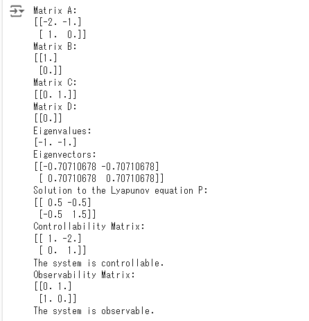
import numpy as np
import scipy.linalg
import scipy.signal as signal
import matplotlib.pyplot as plt
# Transfer function coefficients
a, b, c = 1.0, 2.0, 1.0 # Example values: a=1, b=2, c=1
# Define the transfer function
num = [1]
den = [a, b, c]
system = signal.TransferFunction(num, den)
# Convert to state-space representation
A, B, C, D = signal.tf2ss(num, den)
print("Matrix A:")
print(A)
print("Matrix B:")
print(B)
print("Matrix C:")
print(C)
print("Matrix D:")
print(D)
# Check if the matrix is regular (diagonalization)
eigvals, eigvecs = np.linalg.eig(A)
print("Eigenvalues:")
print(eigvals)
print("Eigenvectors:")
print(eigvecs)
# Solve the Lyapunov equation
Q = np.eye(A.shape[0])
P = scipy.linalg.solve_continuous_lyapunov(A, -Q)
print("Solution to the Lyapunov equation P:")
print(P)
# Check controllability
controllability_matrix = np.hstack([B, np.dot(A, B)])
print("Controllability Matrix:")
print(controllability_matrix)
controllable = np.linalg.matrix_rank(controllability_matrix) == A.shape[0]
print(f"The system is {'controllable' if controllable else 'not controllable'}.")
# Check observability
observability_matrix = np.vstack([C, np.dot(C, A)])
print("Observability Matrix:")
print(observability_matrix)
observable = np.linalg.matrix_rank(observability_matrix) == A.shape[0]
print(f"The system is {'observable' if observable else 'not observable'}.")
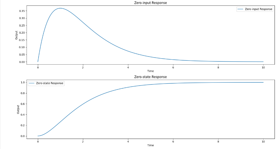
# Time settings for simulation
t = np.linspace(0, 10, 1000)
# Initial state
x0 = [1, 0] # Example initial state [1, 0]
# Zero-input response
_, y_zero_input, x_zero_input = signal.lsim((A, B, C, D), U=0, T=t, X0=x0)
# Zero-state response
u = np.ones_like(t)
_, y_zero_state, x_zero_state = signal.lsim((A, B, C, D), U=u, T=t, X0=0)
# Plotting
plt.figure(figsize=(14, 8))
# Plot zero-input response
plt.subplot(2, 1, 1)
plt.plot(t, y_zero_input, label='Zero-input Response')
plt.xlabel('Time')
plt.ylabel('Output')
plt.title('Zero-input Response')
plt.legend()
# Plot zero-state response
plt.subplot(2, 1, 2)
plt.plot(t, y_zero_state, label='Zero-state Response')
plt.xlabel('Time')
plt.ylabel('Output')
plt.title('Zero-state Response')
plt.legend()
plt.tight_layout()
plt.show()
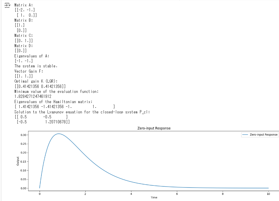
import numpy as np
import scipy.linalg
import scipy.signal as signal
import matplotlib.pyplot as plt

# Transfer function coefficients
a, b, c = 1.0, 2.0, 1.0  # Example values: a=1, b=2, c=1

# Define the transfer function
num = [1]
den = [a, b, c]
system = signal.TransferFunction(num, den)

# Convert to state-space representation
A, B, C, D = signal.tf2ss(num, den)

print("Matrix A:")
print(A)
print("Matrix B:")
print(B)
print("Matrix C:")
print(C)
print("Matrix D:")
print(D)

# Check system stability (Eigenvalues)
eigvals, eigvecs = np.linalg.eig(A)
print("Eigenvalues of A:")
print(eigvals)
stability = np.all(np.real(eigvals) < 0)
print(f"The system is {'stable' if stability else 'unstable'}.")

# Characteristic polynomial and pole placement (vector gain F)
desired_poles = np.array([-1, -2])  # Example desired poles
F = signal.place_poles(A, B, desired_poles).gain_matrix
print("Vector Gain F:")
print(F)

# Optimal regulator (LQR)
Q = np.eye(A.shape[0])
R = np.eye(B.shape[1])
P = scipy.linalg.solve_continuous_are(A, B, Q, R)
K = np.linalg.inv(R).dot(B.T).dot(P)
print("Optimal gain K (LQR):")
print(K)

# Minimum value of the evaluation function
min_eval_func_value = np.trace(P.dot(Q))
print("Minimum value of the evaluation function:")
print(min_eval_func_value)

# Eigenvalues of the Hamiltonian matrix
H = np.block([[A, -B.dot(np.linalg.inv(R)).dot(B.T)], [-Q, -A.T]])
hamilton_eigvals = np.linalg.eigvals(H)
print("Eigenvalues of the Hamiltonian matrix:")
print(hamilton_eigvals)

# Stability of the closed-loop system using the Lyapunov equation
A_cl = A - B.dot(K)
P_cl = scipy.linalg.solve_continuous_lyapunov(A_cl, -Q)
print("Solution to the Lyapunov equation for the closed-loop system P_cl:")
print(P_cl)

# Time settings for simulation
t = np.linspace(0, 10, 1000)

# Initial state
x0 = [1, 0]  # Example initial state [1, 0]

# Zero-input response
_, y_zero_input, x_zero_input = signal.lsim((A_cl, B, C, D), U=0, T=t, X0=x0)

# Zero-state response
u = np.ones_like(t)
_, y_zero_state, x_zero_state = signal.lsim((A_cl, B, C, D), U=u, T=t, X0=0)

# Plotting
plt.figure(figsize=(14, 8))

# Plot zero-input response
plt.subplot(2, 1, 1)
plt.plot(t, y_zero_input, label='Zero-input Response')
plt.xlabel('Time')
plt.ylabel('Output')
plt.title('Zero-input Response')
plt.legend()

# Plot zero-state response
plt.subplot(2, 1, 2)
plt.plot(t, y_zero_state, label='Zero-state Response')
plt.xlabel('Time')
plt.ylabel('Output')
plt.title('Zero-state Response')
plt.legend()

plt.tight_layout()
plt.show()
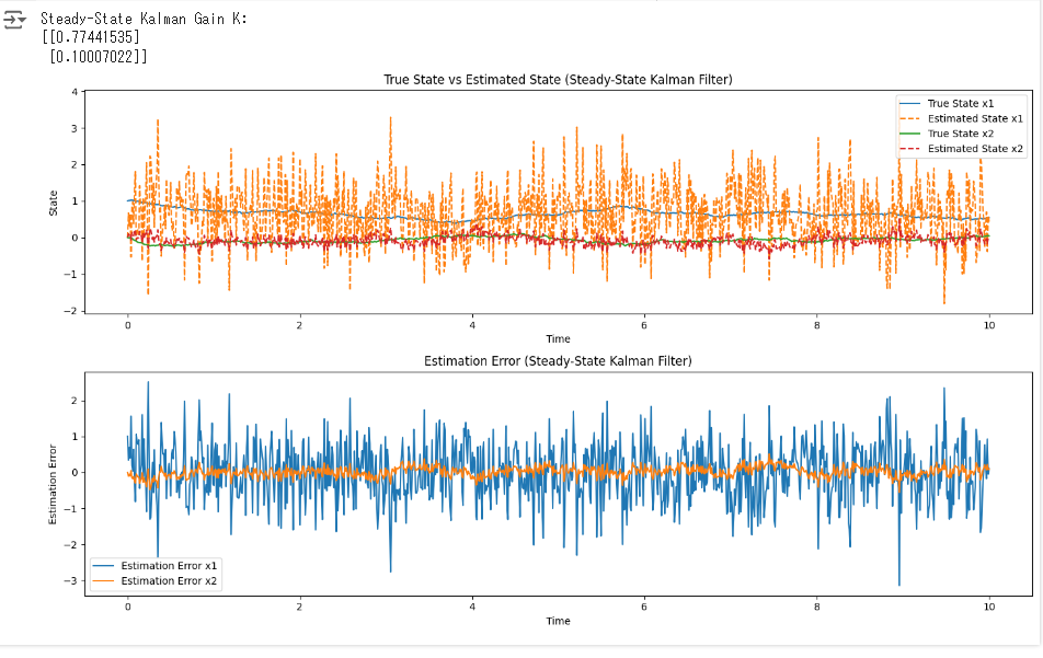
import numpy as np
import scipy.linalg
import scipy.signal as signal
import matplotlib.pyplot as plt

# System parameters
A = np.array([[0, 1], [-2, -3]])  # State matrix
B = np.array([[0], [1]])          # Input matrix
C = np.array([[1, 0]])            # Output matrix
D = np.array([[0]])               # Feedforward matrix

# Noise parameters
Q = np.array([[1, 0], [0, 1]])  # Process noise covariance
R = np.array([[1]])             # Measurement noise covariance

# Calculate steady-state Kalman gain using the discrete-time algebraic Riccati equation
P = scipy.linalg.solve_continuous_are(A, C.T, Q, R)
K = P @ C.T @ np.linalg.inv(R)

print("Steady-State Kalman Gain K:")
print(K)

# Time settings for simulation
t = np.linspace(0, 10, 1000)
dt = t[1] - t[0]

# System noise and measurement noise
np.random.seed(42)  # For reproducibility
process_noise = np.random.normal(0, np.sqrt(Q[0, 0]), size=(len(t), 2))
measurement_noise = np.random.normal(0, np.sqrt(R[0, 0]), len(t))

# Initial states
x = np.zeros((len(t), 2))         # True state
x_hat = np.zeros((len(t), 2))     # Estimated state
x[0] = [1, 0]                     # Initial true state
x_hat[0] = [0, 0]                 # Initial estimated state

# Input signal
u = np.ones_like(t)  # Example input

# State estimation with steady-state Kalman filter
for i in range(1, len(t)):
    # True state update
    x[i] = x[i-1] + (A @ x[i-1] + B.flatten() * u[i-1]) * dt + process_noise[i-1] * dt

    # Measurement update
    y = C @ x[i] + measurement_noise[i]

    # Prediction
    x_hat_minus = x_hat[i-1] + (A @ x_hat[i-1] + B.flatten() * u[i-1]) * dt

    # Update
    x_hat[i] = x_hat_minus + K.flatten() * (y - C @ x_hat_minus)

# Plotting results
plt.figure(figsize=(14, 8))

# Plot true state vs estimated state
plt.subplot(2, 1, 1)
plt.plot(t, x[:, 0], label='True State x1')
plt.plot(t, x_hat[:, 0], label='Estimated State x1', linestyle='dashed')
plt.plot(t, x[:, 1], label='True State x2')
plt.plot(t, x_hat[:, 1], label='Estimated State x2', linestyle='dashed')
plt.xlabel('Time')
plt.ylabel('State')
plt.title('True State vs Estimated State (Steady-State Kalman Filter)')
plt.legend()

# Plot estimation error
estimation_error = x - x_hat
plt.subplot(2, 1, 2)
plt.plot(t, estimation_error[:, 0], label='Estimation Error x1')
plt.plot(t, estimation_error[:, 1], label='Estimation Error x2')
plt.xlabel('Time')
plt.ylabel('Estimation Error')
plt.title('Estimation Error (Steady-State Kalman Filter)')
plt.legend()

plt.tight_layout()
plt.show()
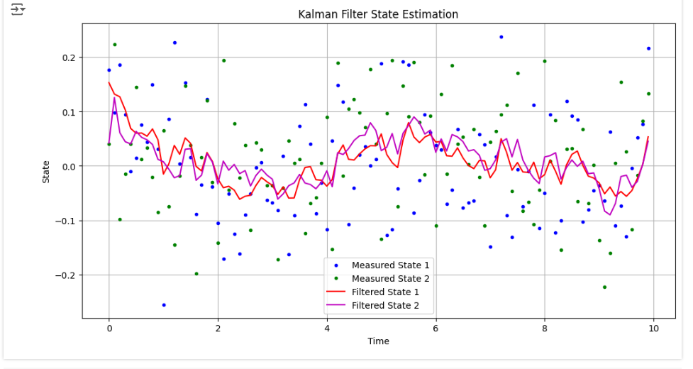
import numpy as np
import matplotlib.pyplot as plt

# カルマンフィルタの実装例
def kalman_filter(A, B, C, Q, R, x0, P0, measurements):
    n = len(A)
    m = len(measurements)

    # 初期化
    x = x0
    P = P0
    filtered_states = []

    for measurement in measurements:
        # 予測ステップ
        x = A @ x
        P = A @ P @ A.T + Q

        # 更新ステップ
        K = P @ C.T @ np.linalg.inv(C @ P @ C.T + R)
        x = x + K @ (measurement - C @ x)
        P = (np.eye(n) - K @ C) @ P

        filtered_states.append(x)

    return np.array(filtered_states)

# テスト用のシステムモデルと外乱
A = np.array([[0.8, 0.2],
              [0.1, 0.9]])
B = np.eye(2)
C = np.eye(2)
Q = np.eye(2) * 0.01  # プロセスノイズ共分散行列
R = np.eye(2) * 0.1   # 観測ノイズ共分散行列

# 初期状態と共分散行列
x0 = np.array([0., 0.])
P0 = np.eye(2)

# ランダムな外乱の生成
np.random.seed(0)
t = np.arange(0, 10, 0.1)
disturbance = 0.1 * np.random.randn(len(t), 2)

# 測定
measurements = np.dot(A, x0) + disturbance

# カルマンフィルタを用いて推定
filtered_states = kalman_filter(A, B, C, Q, R, x0, P0, measurements)

# 結果のプロット
plt.figure(figsize=(12, 6))
plt.plot(t, measurements[:, 0], 'b.', label='Measured State 1')
plt.plot(t, measurements[:, 1], 'g.', label='Measured State 2')
plt.plot(t, filtered_states[:, 0], 'r-', label='Filtered State 1')
plt.plot(t, filtered_states[:, 1], 'm-', label='Filtered State 2')
plt.title('Kalman Filter State Estimation')
plt.xlabel('Time')
plt.ylabel('State')
plt.legend()
plt.grid(True)
plt.show()
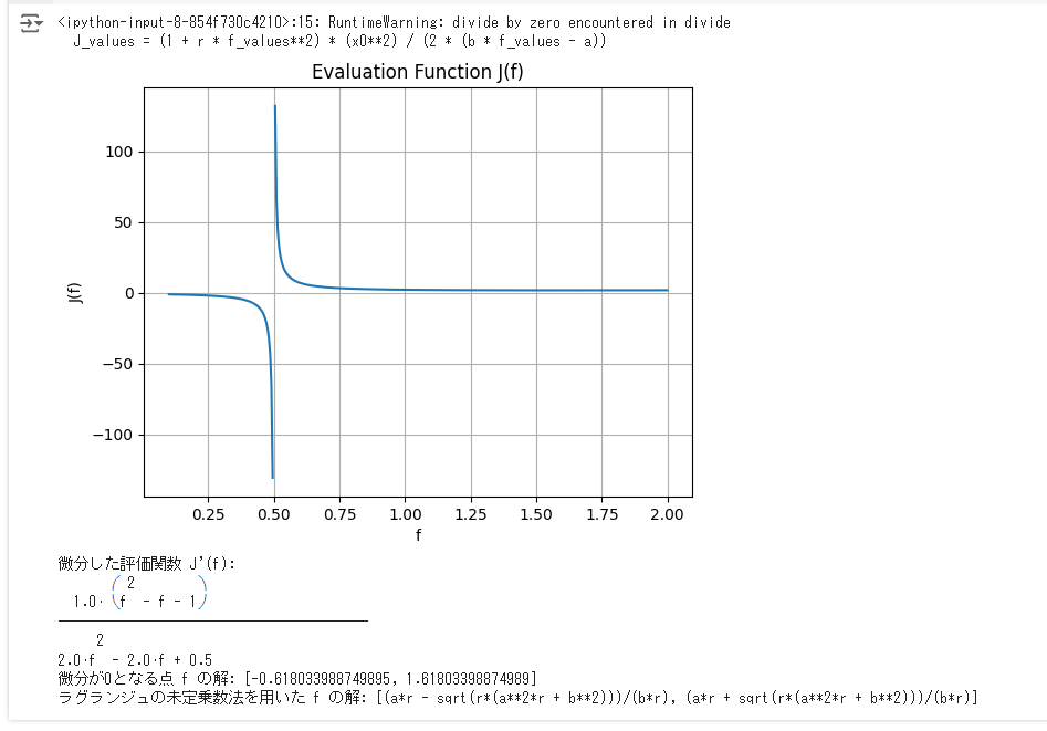
一次遅れ系伝達関数のフィードバックゲインfを求める評価関数
J(f)=(1+rf^2)((x0)^2)/(2(bf-a))
import numpy as np
import matplotlib.pyplot as plt
import sympy as sp

# パラメータの設定
r = 1.0
x0 = 1.0
a = 0.5
b = 1.0

# fの範囲設定
f_values = np.linspace(0.1, 2.0, 400)  # 0.1 から 2.0 までの400点

# 評価関数 J(f) の計算
J_values = (1 + r * f_values**2) * (x0**2) / (2 * (b * f_values - a))

# 評価関数 J(f) のプロット
plt.plot(f_values, J_values)
plt.xlabel('f')
plt.ylabel('J(f)')
plt.title('Evaluation Function J(f)')
plt.grid(True)
plt.show()

# シンボリック変数の定義
f = sp.symbols('f')
J = (1 + r * f**2) * (x0**2) / (2 * (b * f - a))

# 評価関数の微分
J_diff = sp.diff(J, f)
J_diff_simplified = sp.simplify(J_diff)

# 微分した評価関数を表示
print("微分した評価関数 J'(f):")
sp.pretty_print(J_diff_simplified)

# 微分が0となる点を求める
f_solutions = sp.solve(J_diff_simplified, f)
print("微分が0となる点 f の解:", f_solutions)

# ラグランジュの未定乗数法を用いて最小値を求める
# シンボリック変数の定義
f, r, x0, a, b = sp.symbols('f r x0 a b')

# 評価関数の定義
J = (1 + r * f**2) * (x0**2) / (2 * (b * f - a))

# ラグランジュの未定乗数法を用いる
J_diff = sp.diff(J, f)
J_diff_simplified = sp.simplify(J_diff)

# 微分が0となる点を求める
f_solutions = sp.solve(J_diff_simplified, f)
print("ラグランジュの未定乗数法を用いた f の解:", f_solutions)
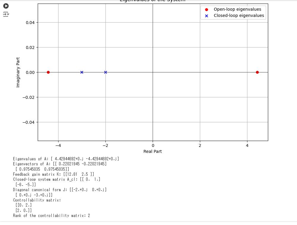
import numpy as np
from scipy.linalg import eig, solve_continuous_are
import matplotlib.pyplot as plt

# Define the parameters
g = 9.81  # acceleration due to gravity (m/s^2)
l = 1.0   # length of the pendulum (m)

# State-space representation
A = np.array([[0, 1], [2*g/l, 0]])
B = np.array([[0], [2/l]])
C = np.array([[1, 0]])
D = np.array([[0]])

# Compute eigenvalues and eigenvectors
eigenvalues, eigenvectors = eig(A)

# Define the desired poles for the closed-loop system
desired_poles = np.array([-2, -3])

# Compute the feedback gain matrix using the pole placement method
from scipy.signal import place_poles
place_obj = place_poles(A, B, desired_poles)
K = place_obj.gain_matrix

# Closed-loop system matrix
A_cl = A - B @ K

# Diagonal canonical form (Jordan form)
eigenvalues_cl, T = eig(A_cl)
J = np.diag(eigenvalues_cl)

# Controllability matrix
ctrb = np.hstack([B, A @ B])
rank_ctrb = np.linalg.matrix_rank(ctrb)

# Plotting eigenvalues
plt.figure(figsize=(10, 6))
plt.scatter(eigenvalues.real, eigenvalues.imag, color='red', marker='o', label='Open-loop eigenvalues')
plt.scatter(eigenvalues_cl.real, eigenvalues_cl.imag, color='blue', marker='x', label='Closed-loop eigenvalues')
plt.axhline(0, color='black', linewidth=0.5)
plt.axvline(0, color='black', linewidth=0.5)
plt.xlabel('Real Part')
plt.ylabel('Imaginary Part')
plt.title('Eigenvalues of the System')
plt.legend()
plt.grid()
plt.show()

# Printing results
print("Eigenvalues of A:", eigenvalues)
print("Eigenvectors of A:", eigenvectors)
print("Feedback gain matrix K:", K)
print("Closed-loop system matrix A_cl:", A_cl)
print("Diagonal canonical form J:", J)
print("Controllability matrix:\n", ctrb)
print("Rank of the controllability matrix:", rank_ctrb)
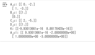
import numpy as np
import scipy.signal as signal
import scipy.linalg as linalg

# 1. 伝達関数の定義
numerator = [1, 5, 3]
denominator = [1, 3, 2]

# 2. 状態空間表現への変換
system = signal.TransferFunction(numerator, denominator)
A, B, C, D = signal.tf2ss(system.num, system.den)

# 3. 制御可能標準形への変換
def controllable_form(A, B, C, D):
    n = A.shape[0]
    cont_matrix = np.hstack([B] + [A**i @ B for i in range(1, n)])
    T = linalg.inv(cont_matrix)
    A_c = T @ A @ np.linalg.inv(T)
    B_c = T @ B
    C_c = C @ np.linalg.inv(T)
    D_c = D
    return A_c, B_c, C_c, D_c

A_c, B_c, C_c, D_c = controllable_form(A, B, C, D)

# 4. 閉ループ極の設定
desired_poles = np.array([-1, -2])

# 5. 状態フィードバックゲインの計算
place = signal.place_poles(A_c, B_c, desired_poles)
K = place.gain_matrix

# 6. 閉ループシステム行列の計算
A_cl = A_c - B_c @ K

# 結果の表示
print("A_c:", A_c)
print("B_c:", B_c)
print("C_c:", C_c)
print("D_c:", D_c)
print("K:", K)
print("A_cl:", A_cl)
import numpy as np
from scipy.signal import place_poles
# 与えられたシステム行列 A, B, C, D を定義する(例として)
A = np.array([[0, 1], [-1, -1]])
B = np.array([[0], [1]])
C = np.array([[1, 0]])
D = np.array([[0]])
# オブザーバーの極を指定する
observer_poles = np.array([-10, -11])
# オブザーバーのゲイン L を求める
L = place_poles(A.T, C.T, observer_poles).gain_matrix.T
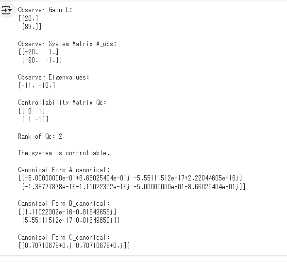
print("Observer Gain L:")
print(L)
# オブザーバーのシステム行列 A_obs を求める
A_obs = A - L @ C
print("\nObserver System Matrix A_obs:")
print(A_obs)
# オブザーバーの極を求める
observer_eigenvalues, _ = np.linalg.eig(A_obs)
print("\nObserver Eigenvalues:")
print(observer_eigenvalues)
# 可制御行列を求める
Qc = np.hstack((B, A @ B))
rank_Qc = np.linalg.matrix_rank(Qc)
print("\nControllability Matrix Qc:")
print(Qc)
print("\nRank of Qc:", rank_Qc)
# 可制御か不可制御かを判定する
if rank_Qc == A.shape[0]:
print("\nThe system is controllable.")
else:
print("\nThe system is uncontrollable.")
# 対角変換行列を求める
eigenvalues, T = np.linalg.eig(A)
T_inv = np.linalg.inv(T)
# 対角正準形に変換する
A_canonical = T_inv @ A @ T
B_canonical = T_inv @ B
C_canonical = C @ T
print("\nCanonical Form A_canonical:")
print(A_canonical)
print("\nCanonical Form B_canonical:")
print(B_canonical)
print("\nCanonical Form C_canonical:")
print(C_canonical)
import numpy as np
import matplotlib.pyplot as plt
# 対角正準形の状態方程式パラメータを設定する(例として)
A_canonical = np.array([[0, 1], [-1, -1]]) # A行列
B_canonical = np.array([[0], [1]]) # B行列
C_canonical = np.array([[1, 0]]) # C行列
D_canonical = np.array([[0]]) # D行列
# 制御対象の状態方程式を定義する
A_sys = A_canonical.copy()
B_sys = B_canonical.copy()
C_sys = C_canonical.copy()
D_sys = D_canonical.copy()
# オブザーバの設計
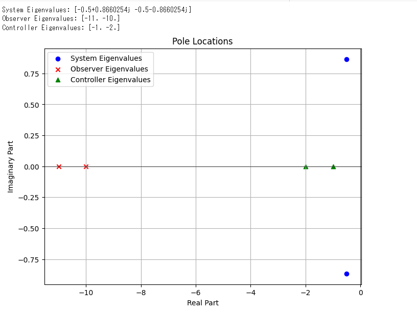
observer_poles = np.array([-10, -11])
L = np.transpose(place_poles(A_sys.T, C_sys.T, observer_poles).gain_matrix)
# コントローラの設計
controller_poles = np.array([-1, -2])
K = place_poles(A_sys, B_sys, controller_poles).gain_matrix
# 制御対象の極を求める
system_eigenvalues, _ = np.linalg.eig(A_sys)
print("System Eigenvalues:", system_eigenvalues)
# オブザーバの極を求める
observer_eigenvalues, _ = np.linalg.eig(A_sys - L @ C_sys)
print("Observer Eigenvalues:", observer_eigenvalues)
# コントローラの極を求める
controller_eigenvalues, _ = np.linalg.eig(A_sys - B_sys @ K)
print("Controller Eigenvalues:", controller_eigenvalues)
# 極の位置をプロットする
plt.figure(figsize=(8, 6))
plt.scatter(system_eigenvalues.real, system_eigenvalues.imag, marker='o', color='blue', label='System Eigenvalues')
plt.scatter(observer_eigenvalues.real, observer_eigenvalues.imag, marker='x', color='red', label='Observer Eigenvalues')
plt.scatter(controller_eigenvalues.real, controller_eigenvalues.imag, marker='^', color='green', label='Controller Eigenvalues')
plt.axhline(0, color='black', linewidth=0.5)
plt.axvline(0, color='black', linewidth=0.5)
plt.xlabel('Real Part')
plt.ylabel('Imaginary Part')
plt.title('Pole Locations')
plt.legend()
plt.grid(True)
plt.show()
import numpy as np
from scipy.optimize import minimize
# 初期状態 x0、スカラー値として定義する
x0 = 1.0
# システムパラメータを定義する
a = 0.5
b = 2.0
c = 1.0
# 評価関数を定義する(この例では二乗誤差を最小化する)
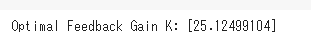
def cost_function(K):
# クローズドループシステムの状態空間表現を定義する
A_cl = a - b * K
B_cl = b
C_cl = c
# 初期状態を定義する
x = np.array([x0])
# シミュレーション時間とステップサイズを定義する
T = 10 # シミュレーション時間
dt = 0.01 # ステップサイズ
time = np.arange(0, T, dt)
# クローズドループのシミュレーションを実行する
for t in time:
u = -K * x[-1] # フィードバック制御則
x_dot = A_cl * x[-1] + B_cl * u
x = np.vstack((x, x[-1] + x_dot * dt))
# 出力を計算する
y = C_cl * x[1:]
# 評価関数を計算する(この例では出力の二乗和を最小化する)
J = np.sum((y - 0)**2) # 目標出力0との差の二乗和
return J
# 初期ゲイン値を設定する
K_initial = 1.0
# 最小化アルゴリズムを使用して最小値を見つける
result = minimize(cost_function, K_initial)
# 最小値を与えるフィードバックゲインを取得する
K_optimal = result.x
print("Optimal Feedback Gain K:", K_optimal)
# プロットするための準備
# フィードバックゲインに対する評価関数の変化をプロットする場合、ここにプロットコードを追加します。
import numpy as np
from scipy.linalg import solve_continuous_are, eig
# 倒立振子モデルのパラメータを定義する
g = 9.81 # 重力加速度 [m/s^2]
l = 1.0 # 振子の長さ [m]
# システムパラメータを定義する
A = np.array([[0, 1], [-2 * g / l, 0]])
B = np.array([[0], [2 / l]])
C = np.array([[1, 0]])
D = np.array([[0]])
# 評価関数の重み行列を設定する
Q = np.eye(2) # 状態の重み行列
R = np.array([[1]]) # 入力の重み行列
# リッカチ方程式の解を計算する
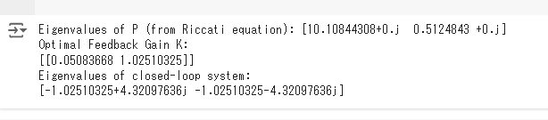
P = solve_continuous_are(A, B, Q, R)
# リッカチ方程式の正定値解を確認する
eigenvalues_P, _ = eig(P)
print("Eigenvalues of P (from Riccati equation):", eigenvalues_P)
# 最適フィードバックゲインを計算する
K_optimal = np.linalg.inv(R) @ B.T @ P
print("Optimal Feedback Gain K:")
print(K_optimal)
# 閉ループシステムのシステム行列を計算する
A_cl = A - B @ K_optimal
# 閉ループシステムの極を計算する
eigenvalues_cl, _ = eig(A_cl)
print("Eigenvalues of closed-loop system:")
print(eigenvalues_cl)
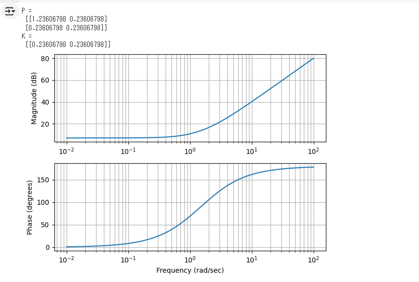
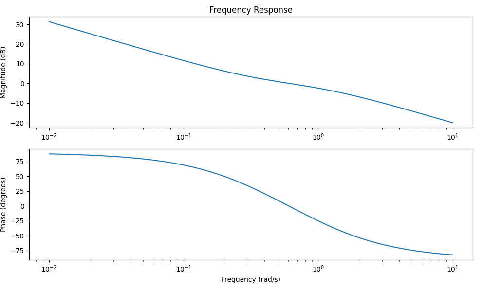
import numpy as np
import scipy.linalg
import matplotlib.pyplot as plt

# システムのパラメータを定義します
A = np.array([[0, 1],
              [-2, -3]])
B = np.array([[0],
              [1]])
Q = np.array([[1, 0],
              [0, 1]])
R = np.array([[1]])

# リッカチ方程式を解きます
P = scipy.linalg.solve_continuous_are(A, B, Q, R)
K = np.linalg.inv(R) @ B.T @ P

# 行列PとKを表示
print("P =\n", P)
print("K =\n", K)

# システムの閉ループ行列を計算します
Acl = A - B @ K

# 周波数特性を計算します
frequencies = np.logspace(-2, 2, 500)
H = np.zeros_like(frequencies, dtype=complex)

for i, w in enumerate(frequencies):
    H[i] = np.linalg.det(1j * w * np.eye(Acl.shape[0]) - Acl)

# 周波数特性をプロットします
magnitude = 20 * np.log10(np.abs(H))
phase = np.angle(H, deg=True)

plt.figure()
plt.subplot(211)
plt.semilogx(frequencies, magnitude)
plt.ylabel('Magnitude (dB)')
plt.grid(which='both', axis='both')

plt.subplot(212)
plt.semilogx(frequencies, phase)
plt.xlabel('Frequency (rad/sec)')
plt.ylabel('Phase (degrees)')
plt.grid(which='both', axis='both')

plt.tight_layout()
plt.show()
import numpy as np
import cvxpy as cp

# システム行列の定義(例としてランダムな行列を使用)
A = np.array([[1.0, 2.0], [-3.0, 4.0]])
B = np.array([[1.0], [0.0]])

# LMI変数の定義
P = cp.Variable((A.shape[0], A.shape[1]), symmetric=True)
Y = cp.Variable((B.shape[1], A.shape[0]))

# LMI条件の設定
constraints = [
    P >> 0,
    A @ P + P @ A.T + B @ Y + Y.T @ B.T << 0
]

# 目的関数(適当に設定)
objective = cp.Minimize(cp.trace(P))

# 最適化問題の定義
prob = cp.Problem(objective, constraints)

# 解を求める
prob.solve()

# 結果の表示
print("P:", P.value)
print("Y:", Y.value)

# 状態フィードバックゲインの計算
K = Y.value @ np.linalg.inv(P.value)
print("状態フィードバックゲイン K:", K)
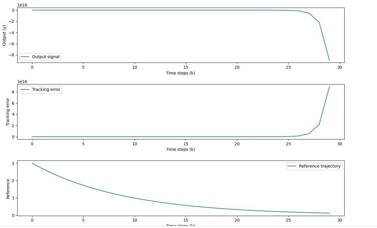
import numpy as np
import matplotlib.pyplot as plt

# Discrete transfer function parameters
b = [2]  # Numerator coefficients
a = [1, -0.7]  # Denominator coefficients

# Sampling period
T = 3  # seconds

# Time vector
k = np.arange(0, 30)  # Assuming 30 time steps

# Reference trajectory: exponential decay with time constant Tref = 9s
Tref = 9
reference = 3 * np.exp(-k / Tref)

# Output signal computation
y = np.zeros_like(k, dtype=float)
u = np.zeros_like(k, dtype=float)

# Initial conditions
y[0] = 2
u[0] = 0.3

for i in range(1, len(k)):
    # Calculate control input u using predictive control law
    if i > 1:
        u[i-1] = b[0] * y[i-1] - a[1] * u[i-2]

    # Simulate the system response
    y[i] = b[0] * u[i-1] + a[1] * y[i-1]

# Plotting
plt.figure(figsize=(12, 8))

plt.subplot(3, 1, 1)
plt.plot(k, y, label='Output signal')
plt.xlabel('Time steps (k)')
plt.ylabel('Output (y)')
plt.legend()

plt.subplot(3, 1, 2)
tracking_error = reference - y[:len(reference)]
plt.plot(k[:len(reference)], tracking_error, label='Tracking error')
plt.xlabel('Time steps (k)')
plt.ylabel('Tracking error')
plt.legend()

plt.subplot(3, 1, 3)
plt.plot(k[:len(reference)], reference, label='Reference trajectory')
plt.xlabel('Time steps (k)')
plt.ylabel('Reference')
plt.legend()

plt.tight_layout()
plt.show()
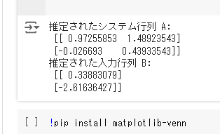
import numpy as np
from scipy.optimize import least_squares

# システムダイナミクスをシミュレートする関数
def simulate_system(A, B, x0, u, noise_std=0.1):
    n = len(x0)
    T = len(u[0])
    x = np.zeros((n, T+1))
    x[:, 0] = x0

    for t in range(T):
        x[:, t+1] = A @ x[:, t] + B @ u[:, t] + np.random.normal(0, noise_std, size=(n,))

    return x[:, :-1], x[:, 1:]

# 最小二乗法を使用して状態空間行列 A と入力行列 B を推定する関数
def estimate_state_space(A_guess, B_guess, y, u):
    n = A_guess.shape[0]
    m = B_guess.shape[1]
    T = y.shape[1]

    def residual(params):
        A_est = params[:n*n].reshape((n, n))
        B_est = params[n*n:].reshape((n, m))

        # 擬似逆行列を使用して初期状態 x0_est を推定
        x0_est = np.linalg.solve(np.eye(n) - A_est, B_est @ u[:, 0])

        # 推定されたパラメータでシステムをシミュレート
        x_sim, _ = simulate_system(A_est, B_est, x0_est, u)

        return (y - x_sim).flatten()

    # パラメータの初期推定値
    init_params = np.concatenate((A_guess.flatten(), B_guess.flatten()))

    # 最小二乗法による最適化
    result = least_squares(residual, init_params)

    # 推定されたシステム行列
    A_est = result.x[:n*n].reshape((n, n))
    B_est = result.x[n*n:].reshape((n, m))

    return A_est, B_est

# 使用例
n = 2  # 状態の数
m = 1  # 入力の数
T = 100  # サンプル数

A_true = np.array([[0.9, 0.1], [0, 0.8]])  # 真のシステム行列
B_true = np.array([[1], [0.5]])  # 真の入力行列
x0_true = np.array([1, 0.5])  # 初期状態ベクトル
u = np.random.randn(m, T)  # ランダムな入力ベクトル

# システムダイナミクスをシミュレートしてサンプルデータを生成
x_true, _ = simulate_system(A_true, B_true, x0_true, u)

# 観測データにノイズを加える
noise_std = 0.1
y = x_true + np.random.normal(0, noise_std, size=x_true.shape)

# システム行列の初期推定値
A_guess = np.random.randn(n, n)
B_guess = np.random.randn(n, m)

# 最小二乗法を使用してシステム行列を推定
A_est, B_est = estimate_state_space(A_guess, B_guess, y, u)

print("推定されたシステム行列 A:\n", A_est)
print("推定された入力行列 B:\n", B_est)
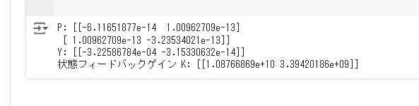
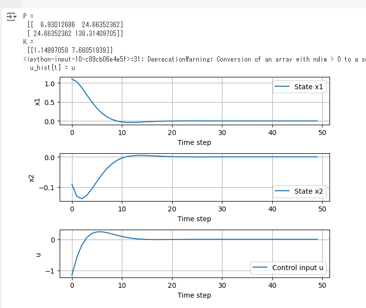
import numpy as np
import matplotlib.pyplot as plt
from scipy.linalg import solve_discrete_are

# System parameters
A = np.array([[1.1, 2], [0, 0.95]])
B = np.array([[0], [0.0787]])
C = np.array([[1, 0]])
Q = np.eye(2)
R = np.eye(1)

# Solve the discrete-time Riccati equation
P = solve_discrete_are(A, B, Q, R)
K = np.linalg.inv(B.T @ P @ B + R) @ (B.T @ P @ A)

# Print the matrices P and K
print("P =\n", P)
print("K =\n", K)

# Simulation parameters
x = np.array([[1], [0]])  # Initial state
n_steps = 50
x_hist = np.zeros((2, n_steps))
u_hist = np.zeros(n_steps)

# Simulation loop
for t in range(n_steps):
    u = -K @ x
    x = A @ x + B @ u
    x_hist[:, t] = x.ravel()
    u_hist[t] = u

# Plot the results
plt.figure()
plt.subplot(311)
plt.plot(x_hist[0, :], label='State x1')
plt.xlabel('Time step')
plt.ylabel('x1')
plt.grid()
plt.legend()

plt.subplot(312)
plt.plot(x_hist[1, :], label='State x2')
plt.xlabel('Time step')
plt.ylabel('x2')
plt.grid()
plt.legend()

plt.subplot(313)
plt.plot(u_hist, label='Control input u')
plt.xlabel('Time step')
plt.ylabel('u')
plt.grid()
plt.legend()

plt.tight_layout()
plt.show()
import numpy as np
import matplotlib.pyplot as plt
from scipy import signal

# Define the Zero-Order Hold (ZOH) as a transfer function in the continuous domain
# ZOH in continuous domain can be approximated as (1 - e^(-sT))/s
T = 1  # Sampling period, example value
zoh_num = [1, -np.exp(-T)]
zoh_den = [T, 0]
zoh_tf = signal.TransferFunction(zoh_num, zoh_den)

# Define the control target transfer function (1/(1 + as))
a = 1  # Example value for a
control_target_tf = signal.TransferFunction([1], [1, a])

# Multiply the transfer functions
# (ZOH * control target) in continuous domain
combined_num = np.polymul(zoh_tf.num, control_target_tf.num)
combined_den = np.polymul(zoh_tf.den, control_target_tf.den)
combined_tf = signal.TransferFunction(combined_num, combined_den)

# Frequency response of the combined system
w, mag, phase = signal.bode(combined_tf)

# Plot the magnitude and phase response
plt.figure(figsize=(10, 6))

plt.subplot(2, 1, 1)
plt.semilogx(w, mag)  # Bode magnitude plot
plt.title('Frequency Response')
plt.ylabel('Magnitude (dB)')

plt.subplot(2, 1, 2)
plt.semilogx(w, phase)  # Bode phase plot
plt.ylabel('Phase (degrees)')
plt.xlabel('Frequency (rad/s)')

plt.tight_layout()
plt.show()
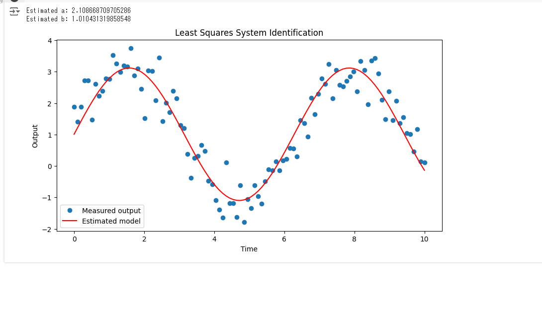
import numpy as np
import matplotlib.pyplot as plt

# Generate synthetic data
np.random.seed(0)
N = 100  # Number of samples
t = np.linspace(0, 10, N)
u = np.sin(t)  # Input signal
a_true = 2.0  # True value of a
b_true = 1.0  # True value of b
noise = 0.5 * np.random.randn(N)  # Gaussian noise
y = a_true * u + b_true + noise  # Output signal

# Least Squares Method for system identification
A = np.vstack([u, np.ones(len(u))]).T
a_est, b_est = np.linalg.lstsq(A, y, rcond=None)[0]

print(f"Estimated a: {a_est}")
print(f"Estimated b: {b_est}")

# Plot results
plt.figure(figsize=(10, 5))
plt.plot(t, y, 'o', label='Measured output')
plt.plot(t, a_est * u + b_est, 'r', label='Estimated model')
plt.legend()
plt.xlabel('Time')
plt.ylabel('Output')
plt.title('Least Squares System Identification')
plt.show()
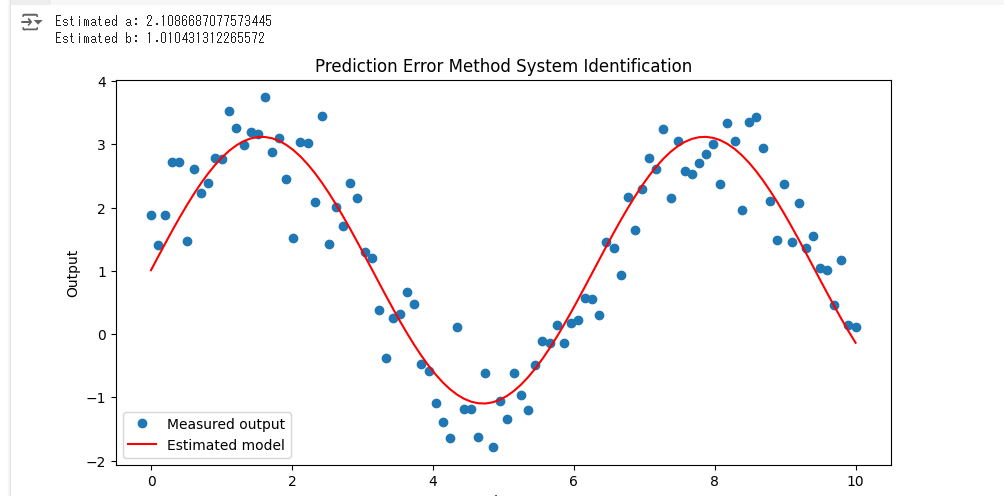
from scipy.optimize import minimize

# Prediction error method for system identification
def prediction_error(params, u, y):
    a, b = params
    y_pred = a * u + b
    error = y - y_pred
    return np.sum(error**2)

# Initial guess for parameters
initial_guess = [1.0, 0.0]

# Perform optimization to minimize the prediction error
result = minimize(prediction_error, initial_guess, args=(u, y))
a_est, b_est = result.x

print(f"Estimated a: {a_est}")
print(f"Estimated b: {b_est}")

# Plot results
plt.figure(figsize=(10, 5))
plt.plot(t, y, 'o', label='Measured output')
plt.plot(t, a_est * u + b_est, 'r', label='Estimated model')
plt.legend()
plt.xlabel('Time')
plt.ylabel('Output')
plt.title('Prediction Error Method System Identification')
plt.show()
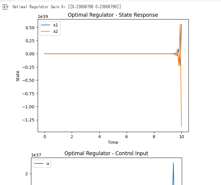
from scipy.linalg import solve_continuous_are

# System matrices
A = np.array([[0, 1], [-2, -3]])
B = np.array([[0], [1]])
Q = np.eye(2)  # State cost matrix
R = np.eye(1)  # Input cost matrix

# Solve Riccati equation
P = solve_continuous_are(A, B, Q, R)

# Optimal gain
K_opt = np.linalg.inv(R).dot(B.T).dot(P)

print("Optimal Regulator Gain K:", K_opt)

# Evaluation function
def cost_function(x, u):
    return x.T.dot(Q).dot(x) + u.T.dot(R).dot(u)

# Plot the state response with the optimal regulator
t = np.linspace(0, 10, 100)
x0 = np.array([1, 0])
x = [x0]
u = []

for _ in t[1:]:
    u_k = -K_opt.dot(x[-1])
    x_k = np.dot(A - np.dot(B, K_opt), x[-1]) + np.dot(B, u_k)
    x.append(x_k)
    u.append(u_k)

x = np.array(x)
u = np.array(u)

plt.figure()
plt.plot(t, x)
plt.title('Optimal Regulator - State Response')
plt.xlabel('Time')
plt.ylabel('State')
plt.legend(['x1', 'x2'])
plt.show()

plt.figure()
plt.plot(t[:-1], u)
plt.title('Optimal Regulator - Control Input')
plt.xlabel('Time')
plt.ylabel('Control Input')
plt.legend(['u'])
plt.show()
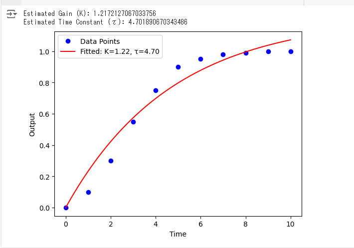
import numpy as np
import matplotlib.pyplot as plt
from scipy.optimize import curve_fit

# Prepare the data
time_data = np.array([0, 1, 2, 3, 4, 5, 6, 7, 8, 9, 10])  # Time data
output_data = np.array([0, 0.1, 0.3, 0.55, 0.75, 0.9, 0.95, 0.98, 0.99, 1.0, 1.0])  # Output data

# Define the first-order system step response function
def first_order_response(t, K, tau):
    return K * (1 - np.exp(-t / tau))

# Initial guess for the parameters
initial_guess = [1.0, 1.0]

# Fit the model to the data using least squares
params, covariance = curve_fit(first_order_response, time_data, output_data, p0=initial_guess)
K_est, tau_est = params

# Display the results
print(f"Estimated Gain (K): {K_est}")
print(f"Estimated Time Constant (τ): {tau_est}")

# Plot the fitting results
plt.plot(time_data, output_data, 'bo', label='Data Points')
time_fit = np.linspace(0, max(time_data), 100)
output_fit = first_order_response(time_fit, K_est, tau_est)
plt.plot(time_fit, output_fit, 'r-', label=f'Fitted: K={K_est:.2f}, τ={tau_est:.2f}')
plt.xlabel('Time')
plt.ylabel('Output')
plt.legend()
plt.show()
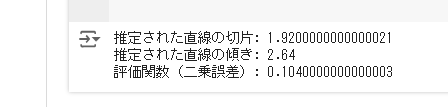
import numpy as np

# サンプルデータ
t = np.array([0, 1, 2, 3, 4])
y = np.array([2.1, 4.3, 7.2, 9.9, 12.5])

# 行列形式に変換
Phi = np.vstack([np.ones_like(t), t]).T

# 重み行列(対角行列を仮定)
W = np.eye(len(t))  # ここでは単位行列を使用

# 最小二乗法による推定
theta_hat = np.linalg.inv(Phi.T @ W @ Phi) @ Phi.T @ W @ y

# 推定されたパラメータ
intercept = theta_hat[0]
slope = theta_hat[1]

# 評価関数(二乗誤差)
J = np.sum((y - Phi @ theta_hat)**2)

print(f"推定された直線の切片: {intercept}")
print(f"推定された直線の傾き: {slope}")
print(f"評価関数(二乗誤差): {J}")
import numpy as np
import matplotlib.pyplot as plt
from scipy.optimize import least_squares
from scipy import signal
from sklearn.datasets import load_iris
from sklearn.naive_bayes import GaussianNB
from sklearn.metrics import accuracy_score
from sklearn.model_selection import train_test_split
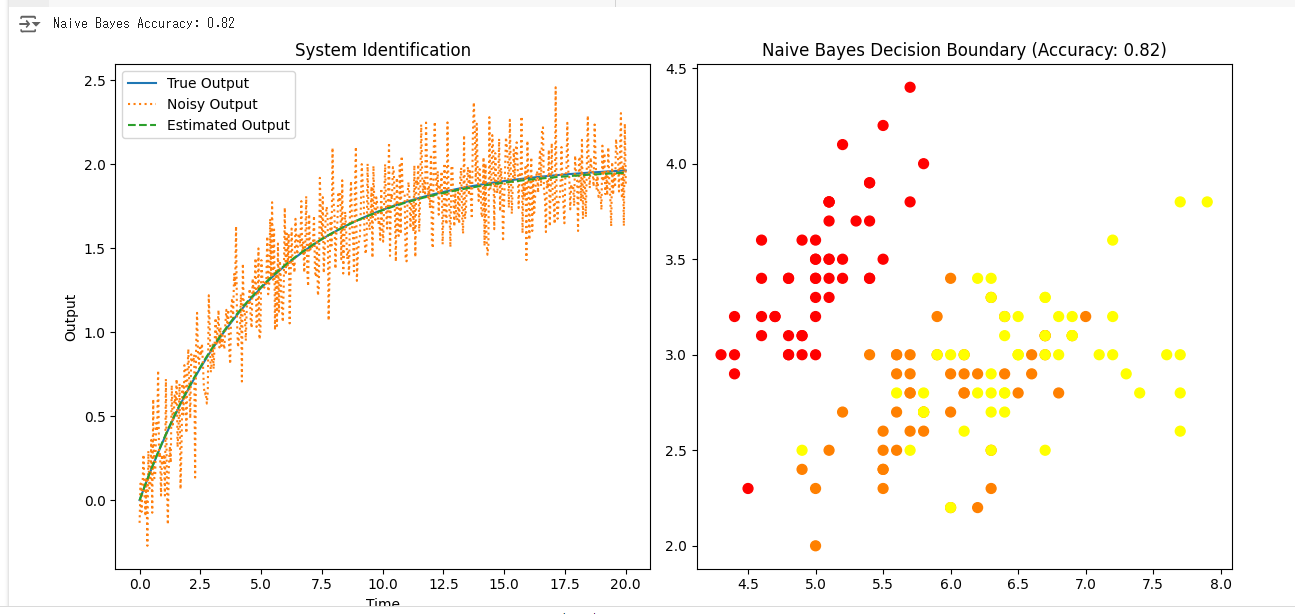
# 1. システム同定
# 真のパラメータ
true_params = [2.0, 5.0] # K, tau
K_true, tau_true = true_params
# 時間軸
t = np.linspace(0, 20, 500)
# ステップ入力
u = np.ones_like(t)
# 一次遅れ系の伝達関数
system = signal.TransferFunction([K_true], [tau_true, 1])
t, y_true = signal.step(system, T=t)
# ノイズを加える
noise = 0.2 * np.random.normal(size=y_true.size)
y_noisy = y_true + noise
# 2. 最小二乗法によるパラメータ推定
def model(params, t, u):
K, tau = params
system = signal.TransferFunction([K], [tau, 1])
_, y = signal.step(system, T=t)
return y
def cost_function(params, t, u, y_noisy):
y_model = model(params, t, u)
return y_noisy - y_model
initial_guess = [1.0, 1.0]
result = least_squares(cost_function, initial_guess, args=(t, u, y_noisy))
estimated_params = result.x
# 推定されたパラメータ
K_est, tau_est = estimated_params
# 推定されたモデル
y_est = model(estimated_params, t, u)
# プロット
plt.figure(figsize=(12, 6))
# システム同定のプロット
plt.subplot(1, 2, 1)
plt.plot(t, y_true, label='True Output')
plt.plot(t, y_noisy, label='Noisy Output', linestyle='dotted')
plt.plot(t, y_est, label='Estimated Output', linestyle='dashed')
plt.xlabel('Time')
plt.ylabel('Output')
plt.legend()
plt.title('System Identification')
# 3. ナイーブベイズ分類器による分類
iris = load_iris()
X = iris.data[:, :2] # 特徴量として2つの変数を使用
y = iris.target
X_train, X_test, y_train, y_test = train_test_split(X, y, test_size=0.3, random_state=42)
gnb = GaussianNB()
gnb.fit(X_train, y_train)
y_pred_nb = gnb.predict(X_test)
# 精度の計算
accuracy_nb = accuracy_score(y_test, y_pred_nb)
print(f'Naive Bayes Accuracy: {accuracy_nb:.2f}')
# ナイーブベイズのプロット
plt.subplot(1, 2, 2)
plt.scatter(X[:, 0], X[:, 1], c=y, s=50, cmap='autumn')
plt.title(f'Naive Bayes Decision Boundary (Accuracy: {accuracy_nb:.2f})')
# グラフのレイアウト調整
plt.tight_layout()
plt.show()
import numpy as np
import matplotlib.pyplot as plt
# 伝達関数の定義
numerator = [1]
denominator = [1, 1, 1]
sys = (numerator, denominator)
# ボード線図をプロットする関数
def bode_plot(sys):
magnitude = []
phase = []
omega = np.logspace(-2, 2, 1000) # ボード線図の周波数範囲を指定
for freq in omega:
s = 1j * freq
G = np.polyval(sys[0], s) / np.polyval(sys[1], s)
magnitude.append(20 * np.log10(abs(G)))
phase.append(np.angle(G, deg=True))
plt.figure()
plt.subplot(2, 1, 1)
plt.semilogx(omega, magnitude)
plt.title('Bode Plot - Magnitude')
plt.grid()
plt.subplot(2, 1, 2)
plt.semilogx(omega, phase)
plt.title('Bode Plot - Phase')
plt.xlabel('Frequency [rad/s]')
plt.grid()
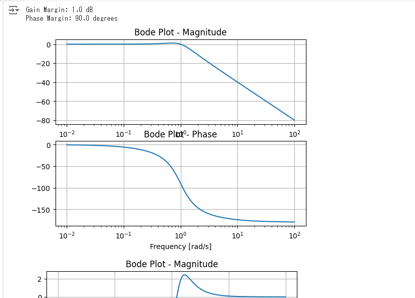
# ロバスト安定性マージンを計算する関数
def stability_margins(sys):
K = np.polyval(sys[0], 0) / np.polyval(sys[1], 0)
L = np.polyder(sys[1])
M = np.polyval(L, 0)
gain_margin = 1 / abs(K)
phase_margin = np.degrees(np.arctan2(M, 1 - K))
return gain_margin, phase_margin
# 相補感度関数を計算してプロットする関数
def complementary_sensitivity(sys):
S_num = sys[1]
S_den = np.polyadd(sys[0], sys[1])
sys_S = (S_num, S_den)
bode_plot(sys_S)
# メインの実行部分
if __name__ == '__main__':
# ボード線図をプロット
bode_plot(sys)
# ロバスト安定性マージンを計算
gm, pm = stability_margins(sys)
print(f"Gain Margin: {gm} dB")
print(f"Phase Margin: {pm} degrees")
# 相補感度関数を計算してプロット
complementary_sensitivity(sys)
plt.show()
import numpy as np
import matplotlib.pyplot as plt

# System transfer function: num/den = 1 / (s^2 + 2s + 1)
num = [1]
den = [1, 2, 1]

# Frequency weight function: W = 1 / (s + 0.5)
W_num = [1]
W_den = [1, 0.5]

# Define the Laplace variable 's'
s = 1j * np.logspace(-1, 1, 1000)

# System transfer function in Laplace domain
G = np.polyval(num, s) / np.polyval(den, s)

# Frequency weight function in Laplace domain
W = np.polyval(W_num, s) / np.polyval(W_den, s)

# Calculate closed-loop transfer function T = KG / (1 + KG)
K = 1 / W  # H-infinity optimal controller K
T = K * G / (1 + K * G)

# Calculate magnitude and phase of T
mag_T = 20 * np.log10(np.abs(T))
phase_T = np.angle(T, deg=True)

# Plot Bode magnitude and phase of T
plt.figure()
plt.subplot(2, 1, 1)
plt.semilogx(np.abs(s), mag_T)
plt.grid(True)
plt.ylabel('Magnitude [dB]')
plt.title('Bode Plot of Closed-loop System with H-infinity Optimal Controller K')

plt.subplot(2, 1, 2)
plt.semilogx(np.abs(s), phase_T)
plt.grid(True)
plt.ylabel('Phase [deg]')
plt.xlabel('Frequency [rad/s]')

plt.tight_layout()
plt.show()
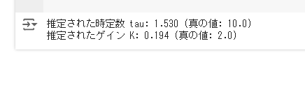
import numpy as np
from sklearn.linear_model import Lasso

# ダミーデータの生成
np.random.seed(0)
N = 100  # データ数
T = 1.0  # サンプリング周期
tau_true = 10.0  # 真の時定数
K_true = 2.0  # 真のゲイン
x_true = np.zeros(N)
u = np.random.randn(N)  # ランダムな入力データ

# 状態方程式のシミュレーション(出力データの生成)
for k in range(N-1):
    x_true[k+1] = (1 - T / tau_true) * x_true[k] + (K_true * T / tau_true) * u[k]
y_true = x_true.copy()  # 出力データは状態ベクトルと同じ

# ノイズの追加
noise_std = 0.1
y = y_true + np.random.randn(N) * noise_std  # ノイズを加えた出力データ

# スパースモデリングによるパラメータ推定
model = Lasso(alpha=0.1)  # Lasso回帰モデルを使用
X = np.column_stack([x_true[:-1], u[:-1]])  # 説明変数の設定
model.fit(X, x_true[1:])  # 状態遷移 x(k+1) の推定

# 推定されたパラメータの表示
tau_estimated = T / model.coef_[0]
K_estimated = model.coef_[1] * tau_estimated / T

print(f"推定された時定数 tau: {tau_estimated:.3f} (真の値: {tau_true})")
print(f"推定されたゲイン K: {K_estimated:.3f} (真の値: {K_true})")
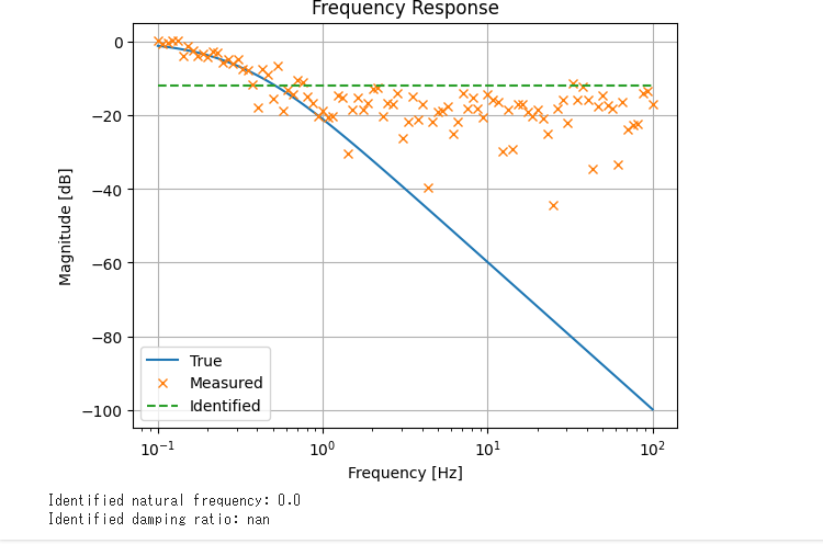
import numpy as np
from sklearn.linear_model import Lasso
import matplotlib.pyplot as plt

# サンプルデータの生成
omega_n_true = 2.0  # 真の自然角周波数
zeta_true = 0.5     # 真の減衰係数
num_points = 100

# 周波数軸の設定
freq = np.logspace(-1, 2, num_points)
omega = 2 * np.pi * freq

# 二次遅れシステムの周波数応答(真の)
H_true = omega_n_true**2 / (omega**2 + 2 * zeta_true * omega_n_true * 1j * omega + omega_n_true**2)

# ノイズを加えた測定データの生成
np.random.seed(0)
noise_level = 0.1
noise = noise_level * (np.random.randn(num_points) + 1j * np.random.randn(num_points))
H_measured = H_true + noise

# データの準備
X = np.vstack((np.real(H_measured), np.imag(H_measured))).T
y = np.abs(H_measured)

# Lasso回帰で係数の同定
lasso = Lasso(alpha=0.1)  # alphaは正則化パラメータ
lasso.fit(X, y)

# 同定された係数
omega_n_identified = np.sqrt(lasso.coef_[0])
zeta_identified = lasso.coef_[1] / (2 * omega_n_identified)

# プロット
plt.figure()
plt.semilogx(freq, 20 * np.log10(np.abs(H_true)), label='True')
plt.semilogx(freq, 20 * np.log10(np.abs(H_measured)), 'x', label='Measured')
plt.semilogx(freq, 20 * np.log10(np.abs(lasso.predict(X))), '--', label='Identified')
plt.xlabel('Frequency [Hz]')
plt.ylabel('Magnitude [dB]')
plt.legend()
plt.grid(True)
plt.title('Frequency Response')
plt.show()

print(f"Identified natural frequency: {omega_n_identified}")
print(f"Identified damping ratio: {zeta_identified}")
import numpy as np
import matplotlib.pyplot as plt
# サンプルデータの準備
T = 10 # シミュレーション時間
dt = 0.01 # サンプリング時間
n = int(T / dt) # サンプル数
# 状態方程式のパラメータ
a = -0.5 # 状態方程式の係数
b = 1.0 # 入力の係数
c = 1.0 # 出力の係数
# 入力信号 (例として単位ステップ関数)
u = np.ones(n)
# サンプルデータから出力を生成
x_true = np.zeros(n)
y_true = np.zeros(n)
for i in range(1, n):
x_true[i] = x_true[i-1] + dt * (a * x_true[i-1] + b * u[i-1])
y_true[i] = c * x_true[i]
# ノイズの追加
noise_std = 0.1 # ノイズの標準偏差
noise = np.random.normal(0, noise_std, n)
y_noisy = y_true + noise
# 状態推定のための最小二乗法
A = np.array([[-a]])
B = np.array([[b]])
C = np.array([[c]])
X_est = np.zeros((1, n)) # 状態推定値の初期化
for i in range(1, n):
X_est[:, i] = X_est[:, i-1] + dt * (A @ X_est[:, i-1].reshape(-1, 1) + B @ u[i-1].reshape(-1, 1)).ravel()
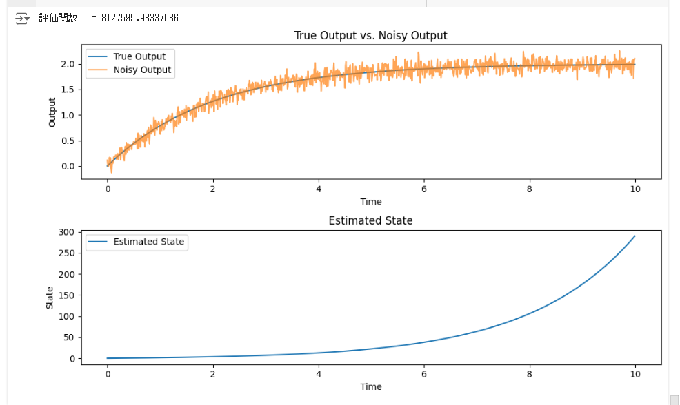
# 評価関数の計算
def cost_function(X_est, Y):
cost = np.sum((C @ X_est - Y) ** 2)
return cost
# 正規方程式の解の計算
Y = y_noisy.reshape(1, -1) # 出力の観測値
# 評価関数の値の表示
J = cost_function(X_est, Y)
print("評価関数 J =", J)
# 結果のプロット
t = np.arange(0, T, dt)
plt.figure(figsize=(10, 6))
plt.subplot(2, 1, 1)
plt.plot(t, y_true, label='True Output')
plt.plot(t, y_noisy, label='Noisy Output', alpha=0.7)
plt.title('True Output vs. Noisy Output')
plt.xlabel('Time')
plt.ylabel('Output')
plt.legend()
plt.subplot(2, 1, 2)
plt.plot(t, X_est.ravel(), label='Estimated State')
plt.title('Estimated State')
plt.xlabel('Time')
plt.ylabel('State')
plt.legend()
plt.tight_layout()
plt.show()
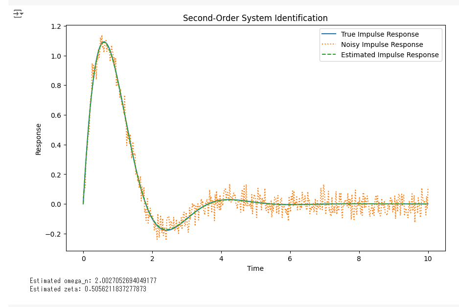
import numpy as np
import matplotlib.pyplot as plt
from scipy.optimize import curve_fit
from scipy.signal import impulse, lti

# 真のパラメータ
omega_n_true = 2.0
zeta_true = 0.5

# インパルス応答を生成する関数
def generate_impulse_response(omega_n, zeta, t):
    system = lti([omega_n**2], [1, 2*zeta*omega_n, omega_n**2])
    t, y = impulse(system, T=t)
    return y

# 時間軸
t = np.linspace(0, 10, 500)

# 真のインパルス応答
y_true = generate_impulse_response(omega_n_true, zeta_true, t)

# システム同定のためのフィッティング関数
def model(t, omega_n, zeta):
    return generate_impulse_response(omega_n, zeta, t)

# ノイズを加える
y_noisy = y_true + 0.05 * np.random.normal(size=t.shape)

# パラメータ推定
popt, pcov = curve_fit(model, t, y_noisy, p0=[1.0, 0.1])
omega_n_est, zeta_est = popt

# 推定されたインパルス応答
y_est = generate_impulse_response(omega_n_est, zeta_est, t)

# 結果をプロット
plt.figure(figsize=(10, 6))
plt.plot(t, y_true, label='True Impulse Response')
plt.plot(t, y_noisy, label='Noisy Impulse Response', linestyle='dotted')
plt.plot(t, y_est, label='Estimated Impulse Response', linestyle='dashed')
plt.legend()
plt.xlabel('Time')
plt.ylabel('Response')
plt.title('Second-Order System Identification')
plt.show()

# 推定結果を表示
print(f"Estimated omega_n: {omega_n_est}")
print(f"Estimated zeta: {zeta_est}")
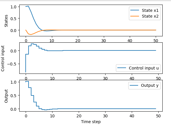
import numpy as np
import matplotlib.pyplot as plt
from scipy.linalg import solve_discrete_are
from scipy.signal import StateSpace, dlti, dstep

# システムの状態空間モデル
A = np.array([[1.1, 2.0], [0, 1.0]])
B = np.array([[0.1], [0.2]])
C = np.array([[1.0, 0.0]])
D = np.array([[0.0]])

# 制御の重み行列
Q = np.eye(2)
R = np.eye(1)

# 無限時間のリカッチ方程式を解く
P = solve_discrete_are(A, B, Q, R)
K = np.linalg.inv(R + B.T @ P @ B) @ (B.T @ P @ A)

# シミュレーションの設定
N = 50  # 時間ステップ数
x = np.zeros((2, N+1))
u = np.zeros((1, N))
y = np.zeros((1, N))
x[:, 0] = [1.0, 0.0]  # 初期状態

# システムのシミュレーション
for k in range(N):
    u[:, k] = -K @ x[:, k]
    x[:, k+1] = A @ x[:, k] + B @ u[:, k]
    y[:, k] = C @ x[:, k]

# 結果のプロット
plt.figure()
plt.subplot(3, 1, 1)
plt.plot(range(N+1), x[0, :], label='State x1')
plt.plot(range(N+1), x[1, :], label='State x2')
plt.ylabel('States')
plt.legend()

plt.subplot(3, 1, 2)
plt.step(range(N), u[0, :], label='Control input u')
plt.ylabel('Control input')
plt.legend()

plt.subplot(3, 1, 3)
plt.step(range(N), y[0, :], label='Output y')
plt.ylabel('Output')
plt.legend()
plt.xlabel('Time step')

plt.show()
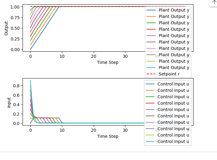
import numpy as np
import matplotlib.pyplot as plt

# プラントパラメータ
A = 1.0
B = 1.0
C = 1.0
D = 0.0

# 制御目標
r = 1.0  # 目標値
N = 10   # 予測ホライズン
T = 50   # シミュレーションステップ数

# MPCパラメータ
Q = 1.0  # 重み行列
R = 0.1  # 重み行列

# 初期化
x = 0.0
u = 0.0
y = 0.0
u_hist = []
y_hist = []

# 参照軌道
ref_trajectory = np.linspace(0, r, N)

for t in range(T):
    # 予測誤差計算
    error = ref_trajectory - y

    # MPC制御則
    BQ = B * Q
    u_opt = (BQ / (R + B * BQ)) * (ref_trajectory - A * x)

    # 入力変化量
    delta_u = u_opt - u
    u = u + delta_u

    # プラント出力計算
    y = A * x + B * u
    x = y  # 状態更新

    # 結果記録
    u_hist.append(u)
    y_hist.append(y)

    # 参照軌道更新
    ref_trajectory = np.roll(ref_trajectory, -1)
    ref_trajectory[-1] = r

# プロット
plt.figure()
plt.subplot(2, 1, 1)
plt.plot(y_hist, label='Plant Output y')
plt.plot([r]*T, 'r--', label='Setpoint r')
plt.xlabel('Time Step')
plt.ylabel('Output')
plt.legend()

plt.subplot(2, 1, 2)
plt.plot(u_hist, label='Control Input u')
plt.xlabel('Time Step')
plt.ylabel('Input')
plt.legend()

plt.tight_layout()
plt.show()
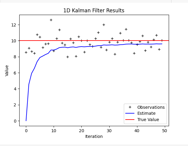
import numpy as np
import matplotlib.pyplot as plt

# Parameters initialization
n_iter = 50  # Number of iterations
true_value = 10  # True value (constant)
z = true_value + np.random.normal(0, 1, n_iter)  # Observations (adding noise)

# Initial estimate
x_hat = np.zeros(n_iter)  # Initialize state estimates
x_hat[0] = 0.0  # Initial state estimate

# Initialize estimate uncertainty
P = np.zeros(n_iter)  # Initialize estimate uncertainty
P[0] = 1.0  # Initial estimate uncertainty

# Measurement uncertainty
R = 1.0  # Measurement uncertainty

# Kalman filter execution
for k in range(1, n_iter):
    # Prediction step
    x_hat[k] = x_hat[k-1]  # State prediction
    P[k] = P[k-1]  # Uncertainty prediction

    # Update step
    K = P[k] / (P[k] + R)  # Compute Kalman gain
    x_hat[k] = x_hat[k] + K * (z[k] - x_hat[k])  # State update
    P[k] = (1 - K) * P[k]  # Uncertainty update

# Plotting results
plt.figure()
plt.plot(z, 'k+', label='Observations')
plt.plot(x_hat, 'b-', label='Estimate')
plt.axhline(true_value, color='r', label='True Value')
plt.legend()
plt.xlabel('Iteration')
plt.ylabel('Value')
plt.title('1D Kalman Filter Results')
plt.show()
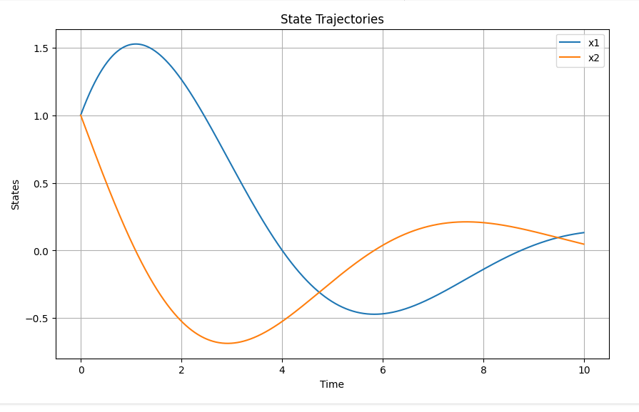
# システム行列 A, B
A = np.array([[0, 1],
              [-1, -1]])
B = np.array([[0],
              [1]])

# リアプノフ関数の重み行列 P (正定値対称行列)
P = np.array([[1, 0],
              [0, 1]])

# 安定化ゲイン alpha
alpha = 1

# シミュレーション時間
T = 10
dt = 0.01
time = np.arange(0, T, dt)

# 状態と入力の初期値
x = np.array([1, 1])  # 初期状態ベクトル
u = 0                 # 初期入力

# 結果の保存用
x_history = np.zeros((len(time), 2))

# シミュレーション
for i in range(len(time)):
    # 状態更新
    x_history[i] = x

    # リアプノフ関数の微分
    V_dot = 2 * np.dot(np.dot(x.T, P), (np.dot(A, x) + np.dot(B, u)))

    # 制御入力計算
    u = -np.dot(np.linalg.inv(B.T @ P @ B + alpha * np.eye(1)), B.T @ P @ A @ x)

    # 状態更新
    x = x + dt * (A @ x + B @ u)

# 結果のプロット
plt.figure(figsize=(10, 6))
plt.plot(time, x_history[:, 0], label='x1')
plt.plot(time, x_history[:, 1], label='x2')
plt.xlabel('Time')
plt.ylabel('States')
plt.title('State Trajectories')
plt.legend()
plt.grid(True)
plt.show()
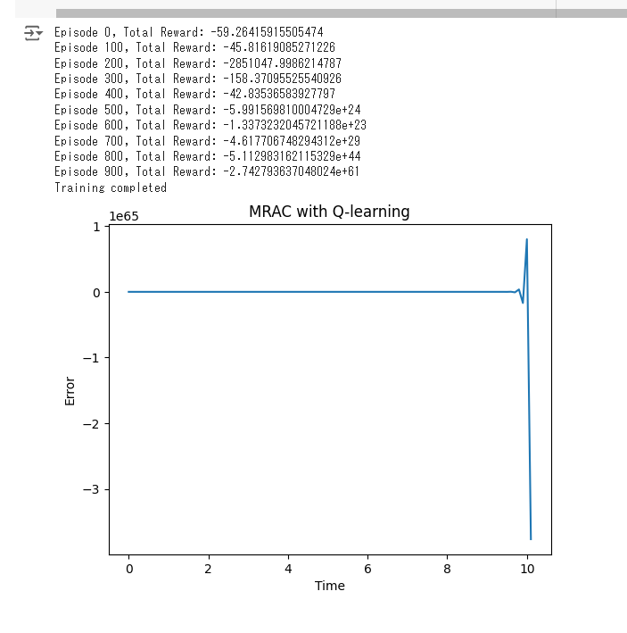
import numpy as np
import matplotlib.pyplot as plt
import gym
from gym import spaces

class SimpleSystemEnv(gym.Env):
    def __init__(self):
        super(SimpleSystemEnv, self).__init__()
        self.observation_space = spaces.Box(low=-np.inf, high=np.inf, shape=(2,), dtype=np.float32)
        self.action_space = spaces.Discrete(3)  # Actions: -1, 0, 1 (change control parameter)
        self.state = np.array([0.0, 0.0])
        self.control_param = 0.5  # Initial control parameter
        self.reference_model = lambda t: np.sin(t)  # Reference model (sine wave)
    def step(self, action):
        t = self.state[0]
        error = self.state[1]
        reference = self.reference_model(t)

        # Update control parameter based on action
        if action == 0:
            self.control_param -= 0.01
        elif action == 2:
            self.control_param += 0.01

        # Simple system dynamics
        control_signal = self.control_param * error
        next_error = reference - control_signal
        self.state = np.array([t + 0.1, next_error])

        reward = -np.abs(next_error)  # Reward is negative absolute error
        done = t >= 10.0  # Episode ends after 10 seconds
        return self.state, reward, done, {}

    def reset(self):
        self.state = np.array([0.0, 0.0])
        return self.state

    def render(self, mode='human'):
        pass

env = SimpleSystemEnv()

# Q-learning parameters
alpha = 0.1  # Learning rate
gamma = 0.99  # Discount factor
epsilon = 0.1  # Exploration rate

q_table = np.zeros((200, 3))  # Q-table initialization

def discretize_state(state):
    t_discrete = int(state[0] * 10)  # Discretize time
    error_discrete = int((state[1] + 1) * 100)  # Discretize error
    return t_discrete, error_discrete

# Training loop
for episode in range(1000):
    state = env.reset()
    total_reward = 0
    done = False
    while not done:
        t_discrete, error_discrete = discretize_state(state)
        if np.random.uniform(0, 1) < epsilon:
            action = env.action_space.sample()  # Exploration
        else:
            action = np.argmax(q_table[t_discrete, :])  # Exploitation

        next_state, reward, done, _ = env.step(action)
        next_t_discrete, next_error_discrete = discretize_state(next_state)

        q_table[t_discrete, action] += alpha * (reward + gamma * np.max(q_table[next_t_discrete, :]) - q_table[t_discrete, action])
        state = next_state
        total_reward += reward

    if episode % 100 == 0:
        print(f"Episode {episode}, Total Reward: {total_reward}")

print("Training completed")

# Test the trained policy
state = env.reset()
done = False
states = []
while not done:
    t_discrete, error_discrete = discretize_state(state)
    action = np.argmax(q_table[t_discrete, :])
    next_state, _, done, _ = env.step(action)
    states.append(state)
    state = next_state

# Plot results
states = np.array(states)
time = states[:, 0]
errors = states[:, 1]
plt.plot(time, errors)
plt.xlabel('Time')
plt.ylabel('Error')
plt.title('MRAC with Q-learning')
plt.show()
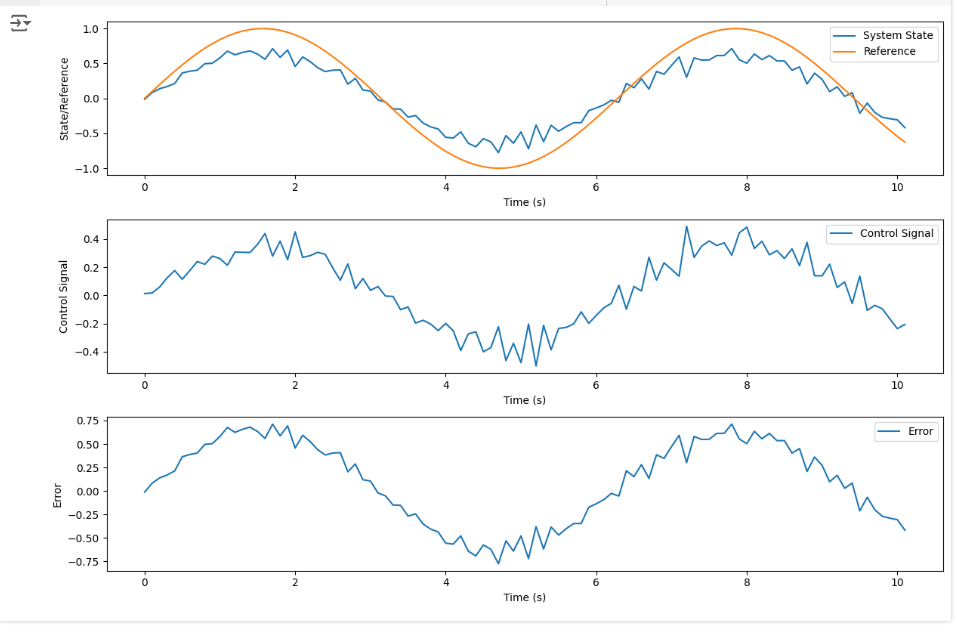
import numpy as np
import gym
import matplotlib.pyplot as plt

class AdaptiveFeedbackControlEnv(gym.Env):
    def __init__(self):
        super(AdaptiveFeedbackControlEnv, self).__init__()
        self.observation_space = spaces.Box(low=-np.inf, high=np.inf, shape=(2,), dtype=np.float32)
        self.action_space = spaces.Discrete(3)  # Actions: -1, 0, 1 (change control parameter)
        self.state = np.array([0.0, 0.0])
        self.control_param = 0.5  # Initial control parameter
        self.reference_model = lambda t: np.sin(t)  # Reference model (sine wave)

    def step(self, action):
        t = self.state[0]
        error = self.state[1]
        reference = self.reference_model(t)

        # Simulate noise affecting the system (example: random noise)
        noise = np.random.normal(loc=0, scale=0.1)
        error_with_noise = error + noise

        # Update control parameter based on action
        if action == 0:
            self.control_param -= 0.01
        elif action == 2:
            self.control_param += 0.01

        # Simple system dynamics with noise
        control_signal = self.control_param * error_with_noise
        next_error = reference - control_signal
        self.state = np.array([t + 0.1, next_error])

        reward = -np.abs(next_error)  # Reward is negative absolute error
        done = t >= 10.0  # Episode ends after 10 seconds
        return self.state, reward, done, {"control_signal": control_signal, "reference": reference, "error": next_error}

    def reset(self):
        self.state = np.array([0.0, 0.0])
        return self.state

    def render(self, mode='human'):
        pass

env = AdaptiveFeedbackControlEnv()

states = []
control_signals = []
references = []
errors = []

state = env.reset()
done = False

while not done:
    action = env.action_space.sample()  # Random action
    state, reward, done, info = env.step(action)
    states.append(state)
    control_signals.append(info['control_signal'])
    references.append(info['reference'])
    errors.append(info['error'])

times = np.arange(0, len(states) * 0.1, 0.1)
states = np.array(states)
control_signals = np.array(control_signals)
references = np.array(references)
errors = np.array(errors)

plt.figure(figsize=(12, 8))
plt.subplot(3, 1, 1)
plt.plot(times, states[:, 1], label='System State')
plt.plot(times, references, label='Reference')
plt.xlabel('Time (s)')
plt.ylabel('State/Reference')
plt.legend()

plt.subplot(3, 1, 2)
plt.plot(times, control_signals, label='Control Signal')
plt.xlabel('Time (s)')
plt.ylabel('Control Signal')
plt.legend()

plt.subplot(3, 1, 3)
plt.plot(times, errors, label='Error')
plt.xlabel('Time (s)')
plt.ylabel('Error')
plt.legend()

plt.tight_layout()
plt.show()
import numpy as np
from scipy.linalg import solve_continuous_are
# システム行列の定義
A1 = np.array([[1.0, 2.0], [-3.0, -4.0]])
A2 = np.array([[0.5, 1.5], [-2.0, -3.5]])
# 任意の対称正定値行列 Q を定義
Q = np.eye(2)
# A1とA2に共通のリアプノフ行列を求める関数
def solve_common_lyapunov(A1, A2, Q):
P1 = solve_continuous_are(A1.T, np.eye(A1.shape[0]), Q, np.eye(A1.shape[0]))
P2 = solve_continuous_are(A2.T, np.eye(A2.shape[0]), Q, np.eye(A2.shape[0]))
P = 0.5 * (P1 + P2)
return P
# 共通リアプノフ行列を計算
P = solve_common_lyapunov(A1, A2, Q)
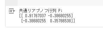
print("共通リアプノフ行列 P:")
print(P)
import numpy as np
import matplotlib.pyplot as plt
# パラメータ設定
dt = 1.0 # タイムステップ
sigma_a = 0.1 # 加速度の標準偏差
sigma_z = 0.1 # 観測誤差の標準偏差
n_steps = 50 # シミュレーションのステップ数
# システム行列
F = np.array([[1, dt], [0, 1]])
G = np.array([[0.5 * dt**2], [dt]])
H = np.array([[1, 0]])
# 共分散行列
Q = sigma_a**2 * np.array([[0.25 * dt**4, 0.5 * dt**3], [0.5 * dt**3, dt**2]])
R = np.array([[sigma_z**2]])
# 初期条件
x = np.array([[0], [0]]) # 初期状態
P = np.zeros((2, 2)) # 初期誤差共分散行列
# カルマンフィルターの結果を保存するリスト
x_estimated = []
x_true = []
z_measurements = []
# シミュレーション
for k in range(n_steps):
# 真の状態更新
a = np.random.normal(0, sigma_a)
w = G * a
x = F @ x + w
x_true.append(x.flatten())
# 観測値
v = np.random.normal(0, sigma_z)
z = H @ x + v
z_measurements.append(z.flatten())
# 予測ステップ
x_pred = F @ x
P_pred = F @ P @ F.T + Q
# 更新ステップ
y = z - H @ x_pred # 観測残差
S = H @ P_pred @ H.T + R # 残差の共分散
K = P_pred @ H.T @ np.linalg.inv(S) # カルマンゲイン
x = x_pred + K @ y
P = (np.eye(2) - K @ H) @ P_pred
x_estimated.append(x.flatten())
# 結果のプロット
x_true = np.array(x_true)
x_estimated = np.array(x_estimated)
z_measurements = np.array(z_measurements)
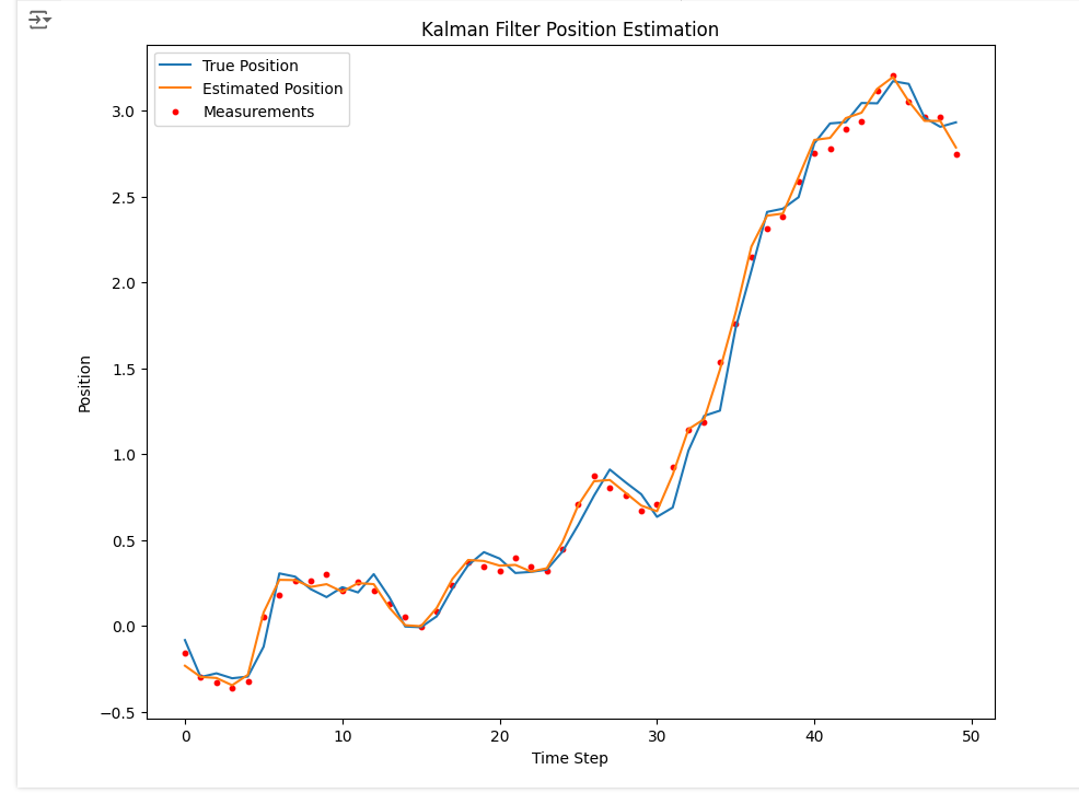
plt.figure(figsize=(10, 8))
plt.plot(x_true[:, 0], label='True Position')
plt.plot(x_estimated[:, 0], label='Estimated Position')
plt.scatter(range(n_steps), z_measurements[:, 0], label='Measurements', color='red', s=10)
plt.xlabel('Time Step')
plt.ylabel('Position')
plt.legend()
plt.title('Kalman Filter Position Estimation')
plt.show()
import numpy as np
import matplotlib.pyplot as plt
from scipy.optimize import minimize
# Parameter settings
T = 0.001 # Sampling period
N = 1000 # Number of simulation steps
prediction_horizon = 20 # Prediction horizon
control_horizon = 5 # Control horizon
s = 1 # Scale of the reference value
tau = 0.1 # Time constant of the reference trajectory
# Weight matrices
Q = 1 # Weight for the output
R = 0.1 # Weight for the input change
# Initialize the discrete integrator
x = 0
y = np.zeros(N)
u = np.zeros(N)
r = np.zeros(N)
# Generate the reference trajectory
for k in range(1, N):
r[k] = s * (1 - np.exp(-k * T / tau))
# Cost function for MPC
def cost_function(U, *args):
y_pred, x0, ref = args
cost = 0
x = x0
for k in range(len(U)):
x = x + U[k]
y_pred[k] = x
cost += Q * (y_pred[k] - ref[k]) ** 2 + R * U[k] ** 2
return cost
# Simulate the system
for k in range(N - prediction_horizon):
# Predict future outputs
y_pred = np.zeros(prediction_horizon)
# Solve the optimization problem
u_initial_guess = np.zeros(control_horizon)
bounds = [(-1, 1)] * control_horizon
res = minimize(cost_function, u_initial_guess, args=(y_pred, x, r[k:k+prediction_horizon]), bounds=bounds)
# Apply the first control input
u[k] = res.x[0]
# Update the state
x = x + u[k]
y[k] = x
# Plot the results
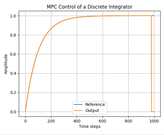
plt.figure()
plt.plot(r, label='Reference')
plt.plot(y, label='Output')
plt.xlabel('Time steps')
plt.ylabel('Amplitude')
plt.legend()
plt.title('MPC Control of a Discrete Integrator')
plt.grid(True)
plt.show()
import numpy as np
# パラメータ推定のためのデータセット
# 例として、xとyのデータが与えられたとします
x = np.array([1, 2, 3, 4, 5])
y = np.array([2.1, 3.9, 6.2, 8.1, 9.8])
# データセットの行列形式
X = np.vstack([np.ones_like(x), x]).T
# データ数
n = len(x)
# 重み行列Wの設定(ここでは単位行列を使用)
W = np.eye(n)
# 最小二乗推定値の計算
theta_hat = np.linalg.inv(X.T @ W @ X) @ X.T @ W @ y
# 評価関数の計算
J = np.sum(W * (y - X @ theta_hat)**2)
# ヘッセ行列の計算(2次形式の係数行列)
Hessian = X.T @ W @ X
# ヘッセ行列が正定値かどうかの確認
is_positive_definite = np.all(np.linalg.eigvals(Hessian) > 0)
# 勾配ベクトルの計算
gradient = -2 * X.T @ W @ (y - X @ theta_hat)
# 結果の出力
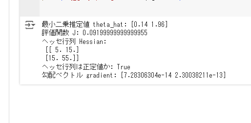
print("最小二乗推定値 theta_hat:", theta_hat)
print("評価関数 J:", J)
print("ヘッセ行列 Hessian:\n", Hessian)
print("ヘッセ行列は正定値か:", is_positive_definite)
print("勾配ベクトル gradient:", gradient)
import numpy as np
import matplotlib.pyplot as plt
from statsmodels.tsa.arima_process import ArmaProcess
from statsmodels.graphics.tsaplots import plot_acf, plot_pacf
# ダミー入力信号の生成(例としてsin波を使う)
t = np.linspace(0, 10, 1000)
input_signal = np.sin(2 * np.pi * t)
# ARMAモデルのパラメータ
order_ar = 2 # AR次数
order_ma = 1 # MA次数
# ARMAモデルの生成
ar_params = np.array([0.5, -0.2]) # AR係数
ma_params = np.array([0.3]) # MA係数
arma_process = ArmaProcess(ar_params, ma_params)
# 入力信号にARMAモデルを適用
arma_signal = arma_process.generate_sample(nsample=len(input_signal))
# 自己相関関数と偏自己相関関数のプロット
fig, (ax1, ax2) = plt.subplots(2, 1, figsize=(10, 8))
plot_acf(arma_signal, ax=ax1, title='Autocorrelation Function (ACF)')
plot_pacf(arma_signal, ax=ax2, title='Partial Autocorrelation Function (PACF)')
plt.tight_layout()
plt.show()
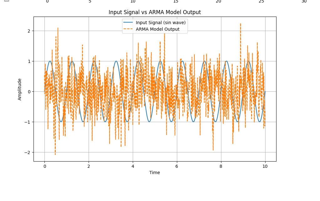
# プロットを使った入力信号とARMAモデルの比較
plt.figure(figsize=(10, 6))
plt.plot(t, input_signal, label='Input Signal (sin wave)')
plt.plot(t, arma_signal, label='ARMA Model Output', linestyle='--')
plt.title('Input Signal vs ARMA Model Output')
plt.xlabel('Time')
plt.ylabel('Amplitude')
plt.legend()
plt.grid(True)
plt.show()
import numpy as np
import matplotlib.pyplot as plt
from scipy.signal import correlate
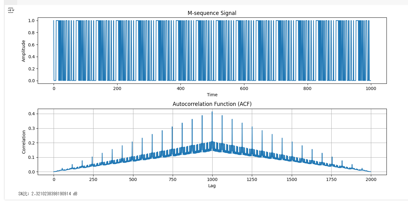
# M系列信号生成関数
def m_sequence(n):
# M系列のレジスタ初期値
register = np.array([1, 0, 0, 0, 0, 0, 0, 1])
sequence = []
for _ in range(n):
sequence.append(register[-1])
new_bit = register[0] ^ register[7] # XORの結果を計算
register = np.roll(register, -1) # レジスタを1ビット左にシフト
register[-1] = new_bit # 新しいビットをレジスタに追加
return np.array(sequence)
# M系列信号の長さ
n = 1000
m_seq = m_sequence(n)
# 自己相関関数の計算
acf = correlate(m_seq, m_seq, mode='full') / n
# SN比の計算(パワー比)
signal_power = np.sum(m_seq ** 2) / n
noise_power = np.sum((m_seq - np.mean(m_seq)) ** 2) / n
snr = 10 * np.log10(signal_power / noise_power)
# プロット:M系列信号と自己相関関数
plt.figure(figsize=(12, 6))
plt.subplot(2, 1, 1)
plt.plot(m_seq)
plt.title('M-sequence Signal')
plt.xlabel('Time')
plt.ylabel('Amplitude')
plt.subplot(2, 1, 2)
plt.plot(acf)
plt.title('Autocorrelation Function (ACF)')
plt.xlabel('Lag')
plt.ylabel('Correlation')
plt.grid(True)
plt.tight_layout()
plt.show()
print(f"SN比: {snr} dB")
import numpy as np
import matplotlib.pyplot as plt

def autocorrelation(signal):
    n = len(signal)
    auto_corr = np.correlate(signal, signal, mode='full') / n
    return auto_corr[n-1:]

def power_spectrum(signal, fs):
    freqs = np.fft.fftfreq(len(signal), d=1/fs)
    psd = np.abs(np.fft.fft(signal))**2 / len(signal)
    return freqs, psd

# 離散時間信号の生成
signal = np.random.randn(100)

# サンプリング周波数
fs = 1  # 1 Hz

# 自己相関関数とパワースペクトル密度関数の計算
auto_corr = autocorrelation(signal)
freqs, psd = power_spectrum(signal, fs)

# プロット
plt.figure(figsize=(12, 4))

# 自己相関関数のプロット
plt.subplot(121)
plt.plot(auto_corr)
plt.title('Autocorrelation Function')
plt.xlabel('Lag')

# パワースペクトル密度関数のプロット
plt.subplot(122)
plt.plot(freqs, psd)
plt.title('Power Spectral Density')
plt.xlabel('Frequency (Hz)')
plt.ylabel('Power')

plt.tight_layout()
plt.show()
import numpy as np
import matplotlib.pyplot as plt
from scipy.integrate import odeint
from sklearn.linear_model import LinearRegression
# システムの定義
def system(y, t, u, Kp, Ki, Kd, setpoint):
e = setpoint - y[0] # 誤差
integral = y[1] # 積分項
derivative = y[2] # 微分項
dydt = [Kp*e + Ki*integral + Kd*derivative, e, y[0]]
return dydt
# システムシミュレーション
def simulate_system(Kp, Ki, Kd, setpoint, disturbance):
t = np.linspace(0, 10, 1000)
y0 = [0, 0, 0] # 初期条件
u = 0
y = odeint(system, y0, t, args=(u, Kp, Ki, Kd, setpoint))
# 外乱を加える
disturbance_signal = disturbance * np.sin(0.1 * np.pi * t)
y[:, 0] += disturbance_signal
return t, y[:, 0]
# データ生成
def generate_data(num_samples):
X = []
y = []
setpoint = 1.0
disturbance = 0.2
for _ in range(num_samples):
Kp = np.random.uniform(0.5, 2.0)
Ki = np.random.uniform(0.1, 1.0)
Kd = np.random.uniform(0.05, 0.5)
t, output = simulate_system(Kp, Ki, Kd, setpoint, disturbance)
error = setpoint - output
mse = np.mean(error**2)
X.append([Kp, Ki, Kd])
y.append(mse)
return np.array(X), np.array(y)
# ゲインのチューニング(機械学習)
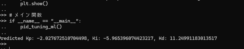
def pid_tuning_ml():
X, y = generate_data(100)
model = LinearRegression()
model.fit(X, y)
# 最適なゲインの予測
Kp, Ki, Kd = model.coef_
print(f"Predicted Kp: {Kp}, Ki: {Ki}, Kd: {Kd}")
setpoint = 1.0
disturbance = 0.2
t, output = simulate_system(Kp, Ki, Kd, setpoint, disturbance)
plt.plot(t, output, label='Output')
plt.axhline(y=setpoint, color='r', linestyle='--', label='Setpoint')
plt.xlabel('Time')
plt.ylabel('Output')
plt.legend()
plt.title('PID Control with Step Input and Disturbance (ML Tuning)')
plt.show()
# メイン関数
if __name__ == "__main__":
pid_tuning_ml()
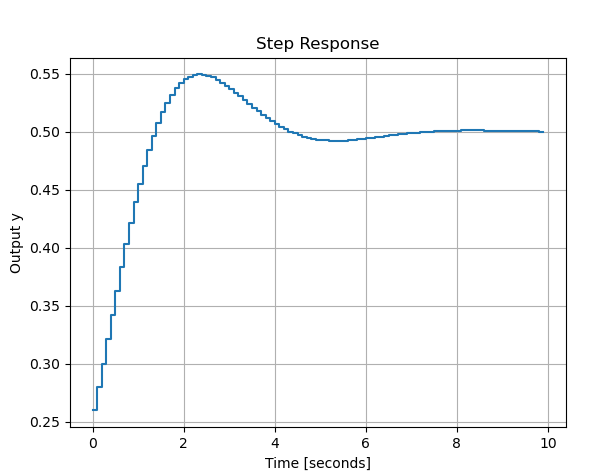
import numpy as np
import scipy.signal as signal
import matplotlib.pyplot as plt

# Continuous-time transfer function coefficients
b0, b1, b2 = 1, 2, 3  # Example coefficients
a0, a1, a2 = 4, 5, 6  # Example coefficients

# Convert transfer function to state-space model
A, B, C, D = signal.tf2ss([b0, b1, b2], [a0, a1, a2])

# Sampling period
T = 0.1  # Example sampling period

# Discretize the system using Tustin (bilinear) transform
system_discrete = signal.cont2discrete((A, B, C, D), T, method='bilinear')

A_d, B_d, C_d, D_d, dt = system_discrete

print("Continuous-time state-space model")
print("A:", A)
print("B:", B)
print("C:", C)
print("D:", D)

print("\nDiscrete-time state-space model")
print("A:", A_d)
print("B:", B_d)
print("C:", C_d)
print("D:", D_d)
print("Sampling period:", dt)

# Simulation of the discrete-time model
# Plot the step response
time_steps = 100  # Number of time steps
u = np.ones(time_steps)
_, y_out, _ = signal.dlsim((A_d, B_d, C_d, D_d, dt), u)

plt.figure()
plt.step(np.arange(time_steps) * T, y_out, where='post')
plt.xlabel('Time [seconds]')
plt.ylabel('Output y')
plt.title('Step Response')
plt.grid()
plt.show()
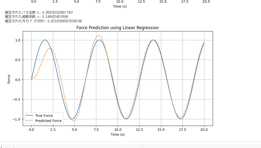
import numpy as np
import matplotlib.pyplot as plt
from scipy.integrate import solve_ivp
from sklearn.linear_model import LinearRegression

# ますばねダンパーのパラメータ
m = 1.0  # 質量
c = 0.5  # 減衰係数
k = 2.0  # バネ定数

# 外力
def external_force(t):
    return np.sin(t)

# 微分方程式
def mass_spring_damper(t, y):
    x, v = y
    F = external_force(t)
    dxdt = v
    dvdt = (F - c * v - k * x) / m
    return [dxdt, dvdt]

# 初期条件
y0 = [0.0, 0.0]  # 初期変位と初速度

# シミュレーション時間
t_span = (0, 20)
t_eval = np.linspace(*t_span, 1000)

# シミュレーション実行
sol = solve_ivp(mass_spring_damper, t_span, y0, t_eval=t_eval)

# シミュレーション結果のプロット
plt.figure(figsize=(10, 5))
plt.plot(sol.t, sol.y[0], label='Position (x)')
plt.plot(sol.t, sol.y[1], label='Velocity (v)')
plt.xlabel('Time (s)')
plt.ylabel('Value')
plt.title('Mass-Spring-Damper System')
plt.legend()
plt.grid()
plt.show()

# 機械学習によるパラメータ調整

# データ生成
X = np.column_stack((sol.y[0], sol.y[1]))  # 変位と速度を特徴量として使用
y = external_force(sol.t)  # 外力をターゲットとして使用

# モデルのトレーニング
model = LinearRegression()
model.fit(X, y)

# モデルの係数と切片
k_pred, c_pred = model.coef_
F_pred = model.intercept_

print(f"推定されたバネ定数 k: {k_pred}")
print(f"推定された減衰係数 c: {c_pred}")
print(f"推定された外力 F の切片: {F_pred}")

# 推定されたモデルによる予測
y_pred = model.predict(X)

# 結果のプロット
plt.figure(figsize=(10, 5))
plt.plot(sol.t, y, label='True Force')
plt.plot(sol.t, y_pred, label='Predicted Force', linestyle='--')
plt.xlabel('Time (s)')
plt.ylabel('Force')
plt.title('Force Prediction using Linear Regression')
plt.legend()
plt.grid()
plt.show()
import numpy as np
import matplotlib.pyplot as plt

# シミュレーションの設定
dt = 1.0  # 時間ステップ(秒)
total_time = 100  # シミュレーション時間(秒)
time = np.arange(0, total_time, dt)

# 真の軌道パラメータ
x_true = 7000.0  # 初期位置 x (km)
y_true = 0.0     # 初期位置 y (km)
vx_true = 0.0    # 初期速度 vx (km/s)
vy_true = 7.5    # 初期速度 vy (km/s)

# 状態ベクトル [x, y, vx, vy]
state_true = np.array([x_true, y_true, vx_true, vy_true])

# 状態遷移行列
F = np.array([[1, 0, dt, 0],
              [0, 1, 0, dt],
              [0, 0, 1, 0],
              [0, 0, 0, 1]])

# 観測行列
H = np.array([[1, 0, 0, 0],
              [0, 1, 0, 0]])

# 観測ノイズの共分散
R = np.diag([100.0, 100.0])  # 観測ノイズの標準偏差を10kmと仮定

# 真の軌道を生成(単純な円軌道を仮定)
true_positions = []
for t in time:
    true_positions.append(state_true[:2])
    state_true = F @ state_true

true_positions = np.array(true_positions)

# ノイズ付き観測データを生成
observed_positions = true_positions + np.random.multivariate_normal([0, 0], R, len(time))

# カルマンフィルタの初期化
state_est = np.array([x_true, y_true, vx_true, vy_true])
P = np.diag([1000.0, 1000.0, 10.0, 10.0])  # 初期共分散行列
Q = np.diag([0.1, 0.1, 0.1, 0.1])  # プロセスノイズの共分散行列

# 推定された位置を保存するリスト
estimated_positions = []

for t in range(len(time)):
    # 時間更新(予測ステップ)
    state_est = F @ state_est
    P = F @ P @ F.T + Q

    # 観測更新(更新ステップ)
    z = observed_positions[t]
    y = z - H @ state_est
    S = H @ P @ H.T + R
    K = P @ H.T @ np.linalg.inv(S)
    state_est = state_est + K @ y
    P = (np.eye(4) - K @ H) @ P

    # 推定された位置を保存
    estimated_positions.append(state_est[:2])

estimated_positions = np.array(estimated_positions)

# 結果のプロット
plt.figure(figsize=(10, 8))
plt.plot(true_positions[:, 0], true_positions[:, 1], label='True Orbit', color='g')
plt.scatter(observed_positions[:, 0], observed_positions[:, 1], label='Observed Position', color='r', s=10)
plt.plot(estimated_positions[:, 0], estimated_positions[:, 1], label='Estimated Orbit', color='b')
plt.xlabel('X position (km)')
plt.ylabel('Y position (km)')
plt.legend()
plt.title('Orbit Estimation using Kalman Filter')
plt.show()
import numpy as np
import matplotlib.pyplot as plt
from scipy.linalg import solve_continuous_are

# 振子のパラメータ
m = 1.0       # 振子の質量 [kg]
l = 1.0       # 振子の長さ [m]
g = 9.81      # 重力加速度 [m/s^2]

# 状態空間モデル
A = np.array([[0, 1],
              [-g/l, 0]])

B = np.array([[0],
              [1/(m*l**2)]])

C = np.array([[1, 0]])

# 重み行列の設定
Q = np.diag([1, 1])   # 状態の重み行列
R = np.array([[1]])  # 入力の重み行列

# リカッチ方程式を解く
P = solve_continuous_are(A, B, Q, R)

# 状態フィードバックゲインを計算
K = np.dot(np.dot(np.linalg.inv(R), B.T), P)

# 初期条件
theta0 = np.pi / 4.0
theta_dot0 = 0.0
x0 = np.array([[theta0], [theta_dot0]])

# シミュレーションパラメータ
dt = 0.02
t_end = 5.0
time = np.arange(0, t_end, dt)
steps = len(time)

# シミュレーション
x_hist = np.zeros((2, steps))
x_hist[:, 0] = x0.flatten()
u_hist = np.zeros(steps)

for i in range(1, steps):
    u = -np.dot(K, x_hist[:, i-1])  # 状態フィードバック制御入力
    u_hist[i] = u  # 制御入力の記録

    # 状態方程式の更新
    x_dot = np.dot(A, x_hist[:, i-1]) + np.dot(B, u)
    x_hist[:, i] = x_hist[:, i-1] + x_dot * dt

# 結果のプロット
plt.figure(figsize=(12, 8))

plt.subplot(3, 1, 1)
plt.plot(time, x_hist[0, :], label='Pendulum Angle')
plt.xlabel('Time (s)')
plt.ylabel('Angle (rad)')
plt.title('Pendulum Angle Control with State Feedback')
plt.legend()
plt.grid(True)

plt.subplot(3, 1, 2)
plt.plot(time, x_hist[1, :], label='Angular Velocity')
plt.xlabel('Time (s)')
plt.ylabel('Angular Velocity (rad/s)')
plt.title('Pendulum Angular Velocity')
plt.legend()
plt.grid(True)

plt.subplot(3, 1, 3)
plt.plot(time, u_hist, label='Control Input (Force)')
plt.xlabel('Time (s)')
plt.ylabel('Control Input (Force)')
plt.title('Control Input (Force) over Time')
plt.legend()
plt.grid(True)

plt.tight_layout()
plt.show()
import numpy as np
import matplotlib.pyplot as plt
from scipy.optimize import minimize

# System parameters
T = 0.1  # Sampling period
tau = 1.0  # Time constant

# Prediction horizon and control horizon
N_pred = 10
N_ctrl = 3

# Constraints
u_min = -1.0
u_max = 1.0

# System model
A = np.exp(-T/tau)
B = (1 - np.exp(-T/tau))

# Target value
r = np.ones(100)  # Step input

# State vector initialization
x = np.zeros(100)
u = np.zeros(100)

# Function to compute optimal input
def cost_function(U, x0, r, N_pred, N_ctrl, A, B):
    x = x0
    cost = 0
    for k in range(N_pred):
        if k < N_ctrl:
            u = U[k]
        else:
            u = U[N_ctrl-1]
        x = A * x + B * u
        cost += (x - r[k])**2
    return cost

# MPC control loop
for k in range(len(r)-N_pred):
    # Set up the optimization problem
    U0 = np.zeros(N_ctrl)  # Initial guess for inputs
    bounds = [(u_min, u_max)] * N_ctrl
    result = minimize(cost_function, U0, args=(x[k], r[k:k+N_pred], N_pred, N_ctrl, A, B), bounds=bounds)
    u[k] = result.x[0]

    # Update the system
    x[k+1] = A * x[k] + B * u[k]

# Plot results separately

# Plot target value and system output
plt.figure()
plt.plot(r, 'r--', label='Target Value')
plt.plot(x, 'b-', label='System Output')
plt.xlabel('Time Step')
plt.ylabel('Value')
plt.legend()
plt.title('System Output vs Target Value')
plt.grid(True)
plt.show()

# Plot control input
plt.figure()
plt.step(np.arange(len(u)), u, 'g-', where='post', label='Control Input')
plt.xlabel('Time Step')
plt.ylabel('Control Input')
plt.legend()
plt.title('Control Input Over Time')
plt.grid(True)
plt.show()
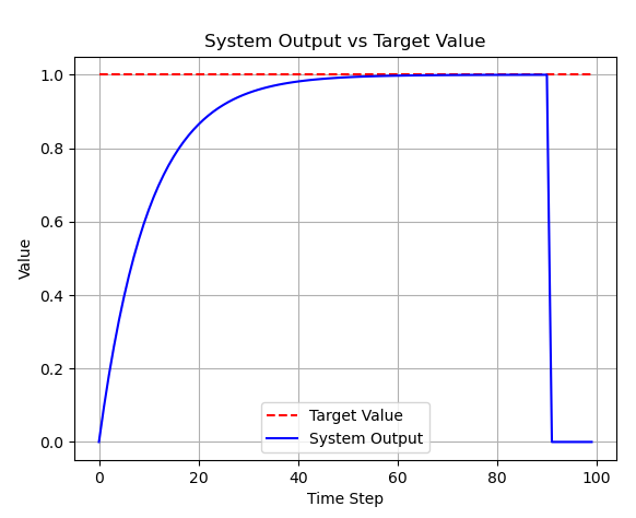
import numpy as np
import matplotlib.pyplot as plt

# 行列の定義
A = np.array([[1, 2],
              [3, 4]])

# 固有値と固有ベクトルの計算
eigenvalues, eigenvectors = np.linalg.eig(A)

print("固有値:", eigenvalues)
print("固有ベクトル:", eigenvectors)

# 状態遷移行列の定義
def plot_phase_portrait(A):
    # グリッドを作成
    x1, x2 = np.meshgrid(np.linspace(-10, 10, 20), np.linspace(-10, 10, 20))
    dx1, dx2 = np.dot(A, np.vstack([x1.ravel(), x2.ravel()]))
    dx1 = dx1.reshape(x1.shape)
    dx2 = dx2.reshape(x2.shape)

    # 位相面図の描画
    plt.figure(figsize=(8, 6))
    plt.quiver(x1, x2, dx1, dx2, angles='xy', scale_units='xy', scale=1, color='r')
    plt.xlim(-10, 10)
    plt.ylim(-10, 10)
    plt.xlabel('x1')
    plt.ylabel('x2')
    plt.title('Phase Portrait')
    plt.grid()
    plt.sho

    w()

# 位相面図を描画
plot_phase_portrait(A)
import numpy as np
from scipy.linalg import solve_continuous_are
import matplotlib.pyplot as plt

# 状態遷移行列 A と正定値行列 Q の定義
A = np.array([[1, 2],
              [3, 4]])
Q = np.eye(2)  # 正定値行列として単位行列を使用

# リアプノフ方程式を解く
P = solve_continuous_are(A, np.eye(2), Q, np.eye(2))

print("リアプノフ行列 P:")
print(P)

# 行列 A の固有値を計算
eigenvalues, _ = np.linalg.eig(A)
print("行列 A の固有値:")
print(eigenvalues)

# 固有値の実部を確認して安定性を判定
if np.all(np.real(eigenvalues) < 0):
    print("システムは漸近的に安定です。")
else:
    print("システムは漸近的に安定ではありません。")

# 位相面図の描画
def plot_phase_portrait(A):
    # グリッドを作成
    x1, x2 = np.meshgrid(np.linspace(-10, 10, 20), np.linspace(-10, 10, 20))
    dx1, dx2 = np.dot(A, np.vstack([x1.ravel(), x2.ravel()]))
    dx1 = dx1.reshape(x1.shape)
    dx2 = dx2.reshape(x2.shape)

    # 位相面図の描画
    plt.figure(figsize=(8, 6))
    plt.quiver(x1, x2, dx1, dx2, angles='xy', scale_units='xy', scale=1, color='r')
    plt.xlim(-10, 10)
    plt.ylim(-10, 10)
    plt.xlabel('x1')
    plt.ylabel('x2')
    plt.title('Phase Portrait')
    plt.grid()
    plt.show()

# 位相面図を描画
plot_phase_portrait(A)
import numpy as np
from scipy.linalg import solve_continuous_are

# システムの定義
A = np.array([[0, 1], [-1, -1]])
B = np.array([[0], [1]])
Q = np.eye(2)  # 状態重み行列
R = np.array([[1]])  # 制御重み行列

# 1. 状態フィードバックゲインの計算(極配置法)
poles = np.array([-2, -3])
# Constructing the controllability matrix
P = np.hstack([np.linalg.matrix_power(A, i) @ B for i in range(A.shape[0])])
# Computing the gain matrix (approximate solution)
K = np.linalg.inv(P.T @ P) @ P.T @ np.array(poles).reshape(-1, 1)
print("State Feedback Gain:", K)

# 2. 最適レギュレータの設計
P_opt = solve_continuous_are(A, B, Q, R)
K_opt = np.linalg.inv(R) @ B.T @ P_opt
print("Optimal State Feedback Gain:", K_opt)

# 3. 固有値の計算
eigenvalues, eigenvectors = np.linalg.eig(A)
print("Eigenvalues:", eigenvalues)

# 4. 初期状態の設定
initial_state = np.array([1, 0])  # 例えば、初期状態が[1, 0]
print("Initial State:", initial_state)

# 5. 対角行列の生成
D = np.diag([1, 2])
print("Diagonal Matrix:", D)

# 6. 評価関数の計算
J = np.trace(P_opt @ Q @ P_opt.T) + np.trace(R)  # 評価関数の例
print("Cost Function:", J)

# 7. リッカチ方程式の解法
P_riccati = solve_continuous_are(A, B, Q, R)
print("Riccati Solution P:", P_riccati)

# 8. ハミルトン行列の生成
H = np.block([[A, np.zeros_like(A)], [-np.linalg.inv(R) @ B @ B.T @ np.linalg.inv(R) @ A.T, -A.T]])
print("Hamiltonian Matrix:", H)

# 9. 可制御性のチェック
P_controllability = np.hstack([np.linalg.matrix_power(A, i) @ B for i in range(A.shape[0])])
controllability_rank = np.linalg.matrix_rank(P_controllability)
print("Controllability Rank:", controllability_rank)

# 10. 可観測性のチェック
C = np.array([[1, 0]])
O = np.vstack([np.linalg.matrix_power(A.T, i) @ C.T for i in range(A.shape[0])]).T
observability_rank = np.linalg.matrix_rank(O)
print("Observability Rank:", observability_rank)
import numpy as np
from scipy.linalg import solve_continuous_are, svd

# システムの定義
A = np.array([[0, 1], [-1, -1]])
B = np.array([[0], [1]])
C = np.array([[1, 0]])
D = np.array([[0]])
Q = np.eye(2)  # 状態重み行列
R = np.array([[1]])  # 制御重み行列

# 1. 状態方程式の定義
# システムの状態方程式は既にA, B, C, Dで定義されています

# 2. 出力フィードバックの設計
P_opt = solve_continuous_are(A, B, Q, R)
K = np.linalg.inv(R) @ B.T @ P_opt
print("Output Feedback Gain K:", K)

# 3. オブザーバーの設計(オブザーバ極の配置)
poles_observer = np.array([-5, -6])  # オブザーバ極の指定
# Constructing the controllability matrix
P_observer = np.hstack([np.linalg.matrix_power(A.T, i) @ C.T for i in range(A.shape[0])]).T
# Computing the observer gain matrix
L = np.linalg.inv(P_observer.T @ P_observer) @ P_observer.T @ np.array(poles_observer).reshape(-1, 1)
print("Observer Gain L:", L)

# 4. 外乱オブザーバの設計(外乱推定のための設計)
A_aug = np.block([[A, np.zeros((A.shape[0], 1))], [np.zeros((1, A.shape[0])), np.array([[0]])]])
B_aug = np.block([[B], [np.array([[1]])]])
C_aug = np.block([[C, np.zeros((C.shape[0], 1))]])
L_aug = np.linalg.inv(P_observer.T @ P_observer) @ P_observer.T @ np.array(poles_observer).reshape(-1, 1)
print("Disturbance Observer Gain L_aug:", L_aug)

# 5. 推定値の計算(例としてステップ応答を用いる)
x0 = np.array([1, 0])  # 初期状態
u = np.array([1])  # 入力信号
dt = 0.01  # タイムステップ
t = np.arange(0, 10, dt)
x = np.zeros((len(t), A.shape[0]))
x_hat = np.zeros((len(t), A.shape[0]))

for i in range(1, len(t)):
    x[i] = x[i-1] + (A @ x[i-1] + B @ u) * dt
    x_hat[i] = x_hat[i-1] + (A @ x_hat[i-1] + B @ u + L @ (C @ (x[i] - x_hat[i-1]))) * dt

print("Estimated State:", x_hat[-1])
import numpy as np
from scipy.linalg import solve_discrete_are

# パラメータの設定
A = np.array([[1, 1], [0, 1]])  # 状態遷移行列
B = np.array([[0.5], [1]])  # 制御行列
C = np.array([[1, 0]])  # 観測行列
Q = np.eye(2)  # プロセスノイズ共分散
R = np.eye(1)  # 観測ノイズ共分散

# 初期値
x_hat = np.array([0, 0])  # 初期推定状態
P = np.eye(2)  # 初期共分散行列

# システムのシミュレーション
np.random.seed(0)
n_steps = 100
true_states = np.zeros((n_steps, 2))
observations = np.zeros(n_steps)
state_noise = np.random.multivariate_normal([0, 0], Q, n_steps)
measurement_noise = np.random.normal(0, np.sqrt(R), n_steps)

for t in range(n_steps):
    if t == 0:
        true_states[t] = x_hat
    else:
        true_states[t] = A @ true_states[t-1] + state_noise[t]
    observations[t] = C @ true_states[t] + measurement_noise[t]

# 推定と評価
estimates = np.zeros((n_steps, 2))
for t in range(n_steps):
    # **予測ステップ**
    x_hat_prior = A @ x_hat
    P_prior = A @ P @ A.T + Q

    # **更新ステップ**
    K = P_prior @ C.T @ np.linalg.inv(C @ P_prior @ C.T + R)  # カルマンゲイン
    x_hat = x_hat_prior + K @ (observations[t] - C @ x_hat)
    P = (np.eye(2) - K @ C) @ P_prior

    # 推定値の保存
    estimates[t] = x_hat

# 推定誤差の2乗平均値を計算
errors = true_states - estimates
mse = np.mean(np.sum(errors**2, axis=1))
print(f'Mean Squared Error: {mse}')

# 共分散行列とリッカチ方程式の解を表示
P_ss = solve_discrete_are(A, B, Q, R)
print(f'Steady-State Covariance Matrix: {P_ss}')
import numpy as np
import matplotlib.pyplot as plt

# Parameters
k = 1.0  # Spring constant
b = 0.1  # Damping constant
m = 1.0  # Mass
dt = 0.01  # Time step
time = np.arange(0, 10, dt)  # Time array

# Initial conditions
theta = np.zeros_like(time)  # Angle
omega = np.zeros_like(time)  # Angular velocity
torque = np.sin(time)  # Input torque (e.g., sine wave)

# Linear model simulation
theta_linear = np.zeros_like(time)
omega_linear = np.zeros_like(time)
for i in range(1, len(time)):
    alpha = (torque[i-1] - b * omega_linear[i-1] - k * theta_linear[i-1]) / m
    omega_linear[i] = omega_linear[i-1] + alpha * dt
    theta_linear[i] = theta_linear[i-1] + omega_linear[i] * dt

# Nonlinear model simulation
theta_nonlinear = np.zeros_like(time)
omega_nonlinear = np.zeros_like(time)
for i in range(1, len(time)):
    friction = 0.1 * omega_nonlinear[i-1]**3  # Nonlinear friction
    alpha = (torque[i-1] - b * omega_nonlinear[i-1] - k * theta_nonlinear[i-1] - friction) / m
    omega_nonlinear[i] = omega_nonlinear[i-1] + alpha * dt
    theta_nonlinear[i] = theta_nonlinear[i-1] + omega_nonlinear[i] * dt

# Plotting results
plt.figure(figsize=(14, 6))

# Linear model results
plt.subplot(1, 2, 1)
plt.plot(time, theta_linear, label='Angle')
plt.plot(time, omega_linear, label='Angular Velocity')
plt.title('Linear Model')
plt.xlabel('Time')
plt.ylabel('Value')
plt.legend()

# Nonlinear model results
plt.subplot(1, 2, 2)
plt.plot(time, theta_nonlinear, label='Angle')
plt.plot(time, omega_nonlinear, label='Angular Velocity')
plt.title('Nonlinear Model')
plt.xlabel('Time')
plt.ylabel('Value')
plt.legend()

plt.tight_layout()
plt.show()
import numpy as np
import scipy.linalg

# システム行列
A = np.array([[1, 1],
              [0, 1]])
B = np.array([[0.5],
              [1.0]])

# コスト行列
Q = np.array([[1, 0],
              [0, 1]])
R = np.array([[1]])

# ホライゾン(制御適用期間)
N = 10

# LQRゲインの計算
def dlqr(A, B, Q, R):
    # Solve the discrete time LQR controller
    X = np.matrix(scipy.linalg.solve_discrete_are(A, B, Q, R))
    K = np.matrix(scipy.linalg.inv(B.T * X * B + R) * (B.T * X * A))
    return np.array(K)

K = dlqr(A, B, Q, R)

# 初期状態
x = np.array([[0],
              [1]])

# システムの挙動をシミュレート
states = [x]
for i in range(N):
    u = -K @ x
    x = A @ x + B @ u
    states.append(x)

# ステージコストと蓄積コスト
stage_costs = []
accumulated_cost = 0
for x in states:
    stage_cost = x.T @ Q @ x
    stage_costs.append(stage_cost.item())
    accumulated_cost += stage_cost.item()

# 結果の表示
print("ステージコスト: ", stage_costs)
print("蓄積コスト: ", accumulated_cost)
print("最終状態: \n", states[-1])
import numpy as np
import matplotlib.pyplot as plt
from scipy.optimize import minimize

# システム行列
A = np.array([[1, 1],
              [0, 1]])
B = np.array([[0.5],
              [1.0]])

# コスト行列
Q = np.array([[1, 0],
              [0, 1]])
R = np.array([[1]])

# 初期状態
x0 = np.array([[0],
               [1]])

# ホライズン(制御適用期間)
N = 10

# 評価関数(総コスト)
def cost_function(u, x0, A, B, Q, R, N):
    u = u.reshape((N, -1))
    x = x0
    total_cost = 0
    for k in range(N):
        u_k = u[k].reshape((-1, 1))
        total_cost += (x.T @ Q @ x + u_k.T @ R @ u_k).item()
        x = A @ x + B @ u_k
    total_cost += (x.T @ Q @ x).item()  # 終端コスト
    return total_cost

# 制約条件(終端時刻の状態をゼロにする)
def terminal_constraint(u, x0, A, B, N):
    u = u.reshape((N, -1))
    x = x0
    for k in range(N):
        u_k = u[k].reshape((-1, 1))
        x = A @ x + B @ u_k
    return x.flatten()

# 初期制御入力(ゼロで初期化)
u0 = np.zeros((N * B.shape[1],))

# 制約の定義
constraints = {'type': 'eq', 'fun': lambda u: terminal_constraint(u, x0, A, B, N)}

# 最適化の実行
result = minimize(cost_function, u0, args=(x0, A, B, Q, R, N), constraints=constraints, method='SLSQP')

# 最適制御入力
optimal_u = result.x.reshape((N, -1))

# システムの挙動をシミュレート
x = x0
states = [x]
for u_k in optimal_u:
    u_k = u_k.reshape((-1, 1))
    x = A @ x + B @ u_k
    states.append(x)

# 結果の表示
print("最適制御入力: \n", optimal_u)
print("最終状態: \n", states[-1])

# ステージコストと蓄積コスト
stage_costs = []
accumulated_cost = 0
for k, x in enumerate(states[:-1]):
    u_k = optimal_u[k].reshape((-1, 1))
    stage_cost = (x.T @ Q @ x + u_k.T @ R @ u_k).item()
    stage_costs.append(stage_cost)
    accumulated_cost += stage_cost
stage_costs.append((states[-1].T @ Q @ states[-1]).item())  # 終端コスト
accumulated_cost += stage_costs[-1]

print("ステージコスト: ", stage_costs)
print("蓄積コスト: ", accumulated_cost)

# グラフのプロット
time = np.arange(N + 1)  # 時間軸(ステップ数)

# 状態のプロット
plt.figure(figsize=(12, 8))

plt.subplot(2, 1, 1)
plt.plot(time, [x[0, 0] for x in states], label='x1')
plt.plot(time, [x[1, 0] for x in states], label='x2')
plt.title('State Trajectories')
plt.xlabel('Time Step')
plt.ylabel('State')
plt.legend()

# 制御入力のプロット
plt.subplot(2, 1, 2)
plt.step(time[:-1], [u[0] for u in optimal_u], where='post')
plt.title('Control Inputs')
plt.xlabel('Time Step')
plt.ylabel('Control Input')
plt.grid()

plt.tight_layout()
plt.show()
import numpy as np
from scipy.optimize import minimize
import matplotlib.pyplot as plt

# 初期状態変数
x0 = np.array([1, 0])  # 例:位置と速度

# システムのパラメータ
A = np.array([[1, 1], [0, 1]])  # 状態遷移行列
B = np.array([[0.5], [1]])      # 入力行列

# 時間ステップ
dt = 1.0
N = 10  # 時間ステップ数

# 評価関数(コスト関数)
def cost(U, x0, A, B, N):
    x = x0
    total_cost = 0
    U = U.reshape(N, 1)  # UをN×1の形に変換
    for i in range(N):
        u = U[i]
        total_cost += np.dot(x.T, x) + u**2  # 二次関数
        x = np.dot(A, x) + np.dot(B, u)
    total_cost += np.dot(x.T, x)  # 終端コスト
    return total_cost

# 最適化するための制御入力の初期値
U0 = np.zeros(N)

# 最適化の制約(ここでは制約なし)
constraints = []

# 最適化実行
result = minimize(cost, U0, args=(x0, A, B, N), constraints=constraints, method='SLSQP')

# 最適化された制御入力
optimal_U = result.x

# システムの挙動をシミュレート
def simulate_system(x0, A, B, U, N):
    x = x0
    states = [x]
    U = U.reshape(N, 1)  # UをN×1の形に変換
    for i in range(N):
        u = U[i]
        x = np.dot(A, x) + np.dot(B, u)
        states.append(x)
    return np.array(states)

# シミュレーションの実行
states = simulate_system(x0, A, B, optimal_U, N)

# プロット
plt.figure(figsize=(12, 8))

# 制御入力のプロット
plt.subplot(2, 1, 1)
plt.plot(range(N), optimal_U, marker='o')
plt.title('Optimal Control Input')
plt.xlabel('Time Step')
plt.ylabel('Control Input')

# 状態のプロット
plt.subplot(2, 1, 2)
plt.plot(range(N+1), states[:, 0], label='Position')
plt.plot(range(N+1), states[:, 1], label='Velocity')
plt.title('System States')
plt.xlabel('Time Step')
plt.ylabel('State')
plt.legend()

plt.tight_layout()
plt.show()
import numpy as np
import matplotlib.pyplot as plt

# パラメータの設定
x_min, x_max = -10, 10
t_min, t_max = 0, 2
dx = 0.1
dt = 0.01

x_values = np.arange(x_min, x_max, dx)
t_values = np.arange(t_min, t_max, dt)

# グリッドの初期化
J = np.zeros((len(t_values), len(x_values)))

# 末端条件の設定
J[-1, :] = np.maximum(0, -x_values**2 + 5)  # 例: 末端条件

# ハミルトニアンの定義
def hamiltonian(x, p, u):
    return 0.5 * (u**2) + p * (x)  # システムダイナミクスに合わせて修正

# 最適制御入力の計算
def optimal_control(p):
    return -p  # ハミルトニアンに合わせて修正

# HJB方程式の数値解法
for t in reversed(range(len(t_values) - 1)):
    for i in range(1, len(x_values) - 1):
        x = x_values[i]
        dJdx = (J[t + 1, i + 1] - J[t + 1, i - 1]) / (2 * dx)

        # 最適制御入力の計算
        u_star = optimal_control(dJdx)

        # ハミルトニアンの評価
        H = hamiltonian(x, dJdx, u_star)

        # HJB方程式の更新
        J[t, i] = J[t + 1, i] + dt * H

# 結果のプロット
X, T = np.meshgrid(x_values, t_values)
plt.contourf(X, T, J, levels=50)
plt.colorbar()
plt.xlabel('x')
plt.ylabel('t')
plt.title('HJB Solution')
plt.show()
import numpy as np
import matplotlib.pyplot as plt
from scipy.integrate import odeint
from scipy.optimize import minimize

# ロトカ・ヴォルテラ方程式
def lotka_volterra(y, t, alpha, beta, delta, gamma, u):
    X1, X2 = y
    dX1dt = alpha * X1 - beta * X1 * X2 + u[0]  # 制御入力uを追加
    dX2dt = delta * X1 * X2 - gamma * X2 + u[1]  # 制御入力uを追加
    return [dX1dt, dX2dt]

# コスト関数
def cost_function(U, y0, t, alpha, beta, delta, gamma, Q, R):
    U = U.reshape((N, 2))
    x = y0
    total_cost = 0
    for i in range(N):
        u = U[i]
        x = odeint(lotka_volterra, x, [t[i], t[i + 1]], args=(alpha, beta, delta, gamma, u))[-1]
        total_cost += np.dot(x, Q @ x) + np.dot(u, R @ u)
    return total_cost

# 制約条件
def control_constraints(U, y0, t, alpha, beta, delta, gamma):
    U = U.reshape((N, 2))
    x = y0
    for i in range(N):
        u = U[i]
        x = odeint(lotka_volterra, x, [t[i], t[i + 1]], args=(alpha, beta, delta, gamma, u))[-1]
    return x - target_state

# パラメータの設定
alpha = 0.1  # 獲物の成長率
beta = 0.02  # 捕食者による獲物の死亡率
delta = 0.01  # 捕食者の繁殖率
gamma = 0.1  # 捕食者の死亡率

# 初期状態と目標状態
X1_0 = 40
X2_0 = 9
y0 = [X1_0, X2_0]
target_state = [20, 5]  # 目標状態

# 時間の設定
t = np.linspace(0, 200, 1000)
dt = t[1] - t[0]
N = 10  # ホライズン

# 初期制御入力(ゼロで初期化)
U0 = np.zeros((N, 2))

# コスト行列
Q = np.eye(2)
R = np.eye(2)

# 制約条件
constraints = {'type': 'eq', 'fun': lambda U: control_constraints(U, y0, t[:N + 1], alpha, beta, delta, gamma)}

# 最適化の実行
result = minimize(cost_function, U0.flatten(), args=(y0, t[:N + 1], alpha, beta, delta, gamma, Q, R), constraints=constraints, method='SLSQP')
optimal_U = result.x.reshape((N, 2))

# シミュレーション
x = y0
states = [x]
for u in optimal_U:
    x = odeint(lotka_volterra, x, [t[0], t[1]], args=(alpha, beta, delta, gamma, u))[-1]
    states.append(x)

states = np.array(states)

# プロット
plt.figure(figsize=(12, 6))

# 獲物の個体数
plt.subplot(2, 1, 1)
plt.plot(t[:N + 1], states[:, 0], label='Prey (X1)')
plt.xlabel('Time')
plt.ylabel('Population')
plt.title('Prey Population with MPC Control')
plt.legend()

# 捕食者の個体数
plt.subplot(2, 1, 2)
plt.plot(t[:N + 1], states[:, 1], label='Predator (X2)', color='r')
plt.xlabel('Time')
plt.ylabel('Population')
plt.title('Predator Population with MPC Control')
plt.legend()

plt.tight_layout()
plt.show()
import numpy as np
import matplotlib.pyplot as plt
from scipy.integrate import solve_ivp

# 定数の定義
alpha = 0.01  # 拡散係数

# 空間の設定
x = np.linspace(0, 10, 100)
dx = x[1] - x[0]

# 初期条件
def initial_condition(x):
    return np.sin(np.pi * x / 10)

u0 = initial_condition(x)

# 時間の設定
t_span = (0, 1)
t_eval = np.linspace(*t_span, 100)

# 偏微分方程式の定義
def heat_equation(t, u_flat):
    u = u_flat.reshape(-1, len(x))
    du_dt = np.zeros_like(u)

    # 2次元のラプラシアン(拡散項)
    du_dt[:, 1:-1] = alpha * (u[:, 2:] - 2 * u[:, 1:-1] + u[:, :-2]) / dx**2

    return du_dt.flatten()

# 初期条件の変換
u0_flat = u0.flatten()

# 方程式の解法
sol = solve_ivp(heat_equation, t_span, u0_flat, t_eval=t_eval, method='RK45')

# 結果のプロット
for i, t in enumerate(sol.t):
    plt.plot(x, sol.y[:, i], label=f't={t:.2f}')

plt.xlabel('x')
plt.ylabel('u(x,t)')
plt.title('Heat Equation Solution')
plt.legend()
plt.show()
# システムの行列を定義します
A = np.array([[0, 1], [-2, -3]])
B = np.array([[0], [1]])
Q = np.eye(2)
R = np.array([[1]])

# リッカチ方程式を解きます
P = solve_continuous_are(A, B, Q, R)

# 最適レギュレータKを計算します
K = inv(R) @ B.T @ P

print("リッカチ行列 P:")
print(P)
print("最適レギュレータ K:")
print(K)
import numpy as np
from scipy.optimize import approx_fprime

# 非線形システムの定義
def f(x, u):
    return np.array([x[0]**2 + x[1]*u, x[1]**2 + u])

# 線形化点
x0 = np.array([1.0, 2.0])
u0 = np.array([0.5])

# ヤコビ行列の計算
def jacobian_f(x, u):
    return approx_fprime(x, lambda x: f(x, u), np.sqrt(np.finfo(float).eps))

A = jacobian_f(x0, u0)
print("状態行列 A:")
print(A)
import numpy as np
import matplotlib.pyplot as plt
from scipy.optimize import minimize

# Objective function
def objective_function(vars):
    x, y = vars
    return x**2 + y**2  # Example objective function to minimize

# Constraint function
def constraint(vars):
    x, y = vars
    return x + y - 1  # Example constraint: x + y = 1

# Initial guess
initial_guess = [0.5, 0.5]

# Define the constraint
constraints = {'type': 'eq', 'fun': constraint}

# Perform the optimization
result = minimize(objective_function, initial_guess, constraints=constraints)

# Extract the results
x_opt, y_opt = result.x
objective_value = result.fun

print("Optimal solution:")
print("x =", x_opt)
print("y =", y_opt)
print("Objective function value =", objective_value)

# Create a grid of (x, y) values
x = np.linspace(-0.5, 1.5, 400)
y = np.linspace(-0.5, 1.5, 400)
X, Y = np.meshgrid(x, y)
Z = X**2 + Y**2

# Plotting
plt.figure(figsize=(12, 6))

# Objective function contour plot
plt.contourf(X, Y, Z, levels=50, cmap='viridis', alpha=0.6)
plt.colorbar(label='Objective function value')

# Constraint line
constraint_x = np.linspace(-0.5, 1.5, 400)
constraint_y = 1 - constraint_x
plt.plot(constraint_x, constraint_y, 'r--', label='x + y = 1')

# Optimal point
plt.plot(x_opt, y_opt, 'bo', label='Optimal solution')

plt.xlabel('x')
plt.ylabel('y')
plt.title('Objective Function and Constraint')
plt.legend()
plt.grid(True)
plt.show()
import numpy as np
import matplotlib.pyplot as plt
from scipy.integrate import odeint

# モデルパラメータ
alpha = 0.33  # 生産関数の弾力性
s = 0.2       # 貯蓄率
delta = 0.05  # 減耗率
K0 = 1.0      # 初期資本ストック

# 生産関数
def production_function(K):
    return K**alpha

# 状態方程式の定義
def model(K, t):
    dKdt = s * production_function(K) - delta * K
    return dKdt

# 時間の設定
t = np.linspace(0, 100, 500)

# 状態方程式の解法
K = odeint(model, K0, t)

# プロット


plt.figure(figsize=(12, 6))
plt.plot(t, K, label='Capital Stock K(t)')
plt.xlabel('Time')
plt.ylabel('Capital Stock')
plt.title('Dynamic Behavior of Capital Stock in Solow Growth Model')
plt.legend()
plt.grid(True)
plt.show()
import numpy as np
import matplotlib.pyplot as plt
from sklearn.linear_model import LinearRegression

# シミュレーションの設定
np.random.seed(0)
T = 100  # 時間ステップ数
t = np.arange(T)  # 時間軸

# 仮のデータ生成(例:経済成長率とインフレーション)
true_slope = 0.5
true_intercept = 2.0
X = t.reshape(-1, 1)  # 説明変数(時間)
y = true_slope * X.flatten() + true_intercept + np.random.normal(0, 1, T)  # 経済指標(データ)

# 線形回帰によるモデルの同定
model = LinearRegression()
model.fit(X, y)

# モデルのパラメータ
estimated_slope = model.coef_[0]
estimated_intercept = model.intercept_

# 将来のデータを生成(例:次の30時間の予測)
future_t = np.arange(T, T + 30).reshape(-1, 1)
future_y = estimated_slope * future_t.flatten() + estimated_intercept

# プロット
plt.figure(figsize=(14, 7))

# 実データと同定結果のプロット
plt.subplot(2, 1, 1)
plt.scatter(t, y, label='Actual Data')
plt.plot(t, model.predict(X), color='r', label='Fitted Line')
plt.xlabel('Time')
plt.ylabel('Economic Indicator')
plt.title('Model Identification')
plt.legend()
plt.grid(True)

# 予測結果のプロット
plt.subplot(2, 1, 2)
plt.plot(np.concatenate([t, future_t.flatten()]),
         np.concatenate([model.predict(X), future_y]),
         color='b', label='Predicted')
plt.axvline(x=T, color='g', linestyle='--', label='Prediction Start')
plt.xlabel('Time')
plt.ylabel('Economic Indicator')
plt.title('Forecast')
plt.legend()
plt.grid(True)

plt.tight_layout()
plt.show()
import numpy as np
from scipy.integrate import odeint
from scipy.optimize import minimize
import matplotlib.pyplot as plt

# ロジスティック成長モデルの微分方程式
def logistic_growth(P, t, r):
    K = 1000  # 環境の収容能力
    dP_dt = r * P * (1 - P / K)
    return dP_dt

# 目的関数
def objective(params):
    r = params[0]  # 成長率
    P0 = 10  # 初期個体数
    P_target = 500  # 目標個体数
    T = 100  # シミュレーションの時間
    t = np.linspace(0, T, 100)

    # 微分方程式の解
    P = odeint(logistic_growth, P0, t, args=(r,))

    # 目的関数の計算 (個体数と目標個体数の差の平方和)
    cost = np.sum((P - P_target) ** 2)
    return cost

# 初期推定
initial_guess = [0.1]

# 最適化
result = minimize(objective, initial_guess, bounds=[(0, None)])

# 結果の表示
optimal_r = result.x[0]
print(f"Optimal growth rate: {optimal_r}")

# 最適な成長率でシミュレーション
P0 = 10
T = 100
t = np.linspace(0, T, 100)
P_optimal = odeint(logistic_growth, P0, t, args=(optimal_r,))

# 結果のプロット
plt.plot(t, P_optimal, label=f'Optimal Growth Rate (r={optimal_r:.2f})')
plt.xlabel('Time')
plt.ylabel('Population')
plt.title('Bacterial Growth with Optimal Control')
plt.legend()
plt.grid(True)
plt.show()
import numpy as np
import matplotlib.pyplot as plt
from scipy.linalg import solve_continuous_are
from scipy.linalg import inv

# システムのパラメータ
k1 = 1.0  # 反応速度定数
A = np.array([[-k1, 0], [k1, 0]])  # 状態遷移行列
B = np.array([[1], [0]])           # 制御行列
Q = np.eye(2)                       # 状態重み行列
R = np.array([[1]])                 # 制御重み行列

# リカッチ方程式を解く
P = solve_continuous_are(A, B, Q, R)

# 最適制御ゲインを計算
K = inv(R) @ B.T @ P

# シミュレーションのパラメータ
T = 10
dt = 0.1
t = np.arange(0, T, dt)
x0 = np.array([10, 0])  # 初期状態
x = np.zeros((len(t), 2))
x[0, :] = x0

# システムのシミュレーション
for i in range(1, len(t)):
    u = -K @ x[i-1, :]  # 最適制御入力
    x[i, :] = x[i-1, :] + (A @ x[i-1, :] + B.flatten() * u) * dt

# 結果のプロット
plt.figure(figsize=(12, 6))

plt.subplot(1, 2, 1)
plt.plot(t, x[:, 0], label='Substrate (S)')
plt.xlabel('Time')
plt.ylabel('Concentration')
plt.title('Substrate Concentration Over Time')
plt.legend()
plt.grid(True)

plt.subplot(1, 2, 2)
plt.plot(t, x[:, 1], label='Product (P)', color='orange')
plt.xlabel('Time')
plt.ylabel('Concentration')
plt.title('Product Concentration Over Time')
plt.legend()
plt.grid(True)

plt.tight_layout()
plt.show()
import numpy as np
import matplotlib.pyplot as plt
from scipy.linalg import solve_continuous_are, inv

# モデルのパラメータ
alpha = np.array([0.1, 0.05, 0.2])  # 状態遷移の減衰係数
beta = np.array([1, 1, 1])          # 制御入力の影響

# 状態遷移行列Aと制御行列Bの設定
A = np.diag(-alpha)
B = np.reshape(beta, (3, 1))
Q = np.eye(3)  # 状態重み行列
R = np.array([[1]])  # 制御重み行列

# リカッチ方程式を解いてPを計算
P = solve_continuous_are(A, B, Q, R)

# 状態フィードバックゲインKの計算
K = inv(R) @ B.T @ P

print("最適状態フィードバックゲイン K:")
print(K)

# シミュレーションのパラメータ
T = 20
dt = 0.1
t = np.arange(0, T, dt)
x0 = np.array([10, 7, 5])  # 初期状態(温度、pH、栄養素濃度)
x = np.zeros((len(t), 3))
x[0, :] = x0

# システムのシミュレーション
for i in range(1, len(t)):
    u = -K @ x[i-1, :]  # 状態フィードバック制御入力
    x[i, :] = x[i-1, :] + (A @ x[i-1, :] + B.flatten() * u) * dt

# 結果のプロット
plt.figure(figsize=(12, 6))

plt.subplot(1, 3, 1)
plt.plot(t, x[:, 0], label='Temperature (T)')
plt.xlabel('Time')
plt.ylabel('Temperature')
plt.title('Temperature Over Time')
plt.legend()
plt.grid(True)

plt.subplot(1, 3, 2)
plt.plot(t, x[:, 1], label='pH (pH)', color='orange')
plt.xlabel('Time')
plt.ylabel('pH')
plt.title('pH Over Time')
plt.legend()
plt.grid(True)

plt.subplot(1, 3, 3)
plt.plot(t, x[:, 2], label='Nutrients (N)', color='green')
plt.xlabel('Time')
plt.ylabel('Nutrients')
plt.title('Nutrients Over Time')
plt.legend()
plt.grid(True)

plt.tight_layout()
plt.show()
import numpy as np
import matplotlib.pyplot as plt

# 擬似的な地震データの生成(例としてランダムデータを使用)
np.random.seed(42)
time = np.arange(0, 100, 1)
earthquake_activity = np.sin(time / 5) + np.random.normal(0, 0.2, len(time))  # ノイズを少なく

# カルマンフィルタのパラメータ設定
n = len(time)
A = 1  # 状態遷移行列
B = 0  # 制御入力行列(今回は制御なし)
H = 1  # 観測行列
Q = 1e-5  # プロセスノイズの共分散(小さく設定)
R = 0.2**2  # 観測ノイズの共分散(小さく設定)

# 初期化
x_hat = np.zeros(n)  # 推定値
P = np.zeros(n)  # 推定誤差共分散
x_hat[0] = earthquake_activity[0]  # 初期推定値
P[0] = 1  # 初期誤差共分散

# カルマンフィルタの適用
for k in range(1, n):
    # 予測ステップ
    x_hat[k] = A * x_hat[k-1] + B
    P[k] = A * P[k-1] * A + Q

    # 更新ステップ
    K = P[k] * H / (H * P[k] * H + R)
    x_hat[k] = x_hat[k] + K * (earthquake_activity[k] - H * x_hat[k])
    P[k] = (1 - K * H) * P[k]

# 結果のプロット
plt.figure(figsize=(12, 6))

plt.plot(time, earthquake_activity, label='Actual Earthquake Activity', color='blue')
plt.plot(time, x_hat, label='Filtered Earthquake Activity', color='red', linestyle='--')
plt.xlabel('Time')
plt.ylabel('Earthquake Activity')
plt.title('Earthquake Activity Prediction with Improved Kalman Filter')
plt.legend()
plt.grid(True)
plt.show()
import numpy as np
import matplotlib.pyplot as plt
from scipy.integrate import odeint

# システムのパラメータ
Kp = 2.0  # 比例ゲイン
Ki = 0.5  # 積分ゲイン
Kd = 0.1  # 微分ゲイン

# PID制御の計算
def pid_control(setpoint, measurement, integral, previous_error, dt):
    error = setpoint - measurement
    integral += error * dt
    derivative = (error - previous_error) / dt
    control_signal = Kp * error + Ki * integral + Kd * derivative
    return control_signal, integral, error

# システムモデルの定義
def system_model(y, t, control_signal):
    dydt = -0.1 * y + control_signal
    return dydt

# シミュレーションのパラメータ
T = 20
dt = 0.1
time = np.arange(0, T, dt)
setpoint = 10
measurement = 0
integral = 0
previous_error = 0

# 結果の保存
y = np.zeros_like(time)
for i in range(len(time)):
    control_signal, integral, previous_error = pid_control(setpoint, measurement, integral, previous_error, dt)
    y[i] = odeint(system_model, measurement, [0, dt], args=(control_signal,))[1]
    measurement = y[i]

# 結果のプロット
plt.plot(time, y, label='Measured Value')
plt.axhline(y=setpoint, color='r', linestyle='--', label='Setpoint')
plt.xlabel('Time')
plt.ylabel('Value')
plt.title('PID Control for Cell Cultivation')
plt.legend()
plt.grid(True)
plt.show()
import numpy as np
from scipy.linalg import solve_continuous_are, inv
import matplotlib.pyplot as plt
from scipy.integrate import solve_ivp

# 状態空間モデルのパラメータ
alpha = 0.1  # 発現量の減衰率
beta = 1.0   # 制御入力の影響

# 状態行列 A と入力行列 B の定義
A = np.array([[-alpha]])
B = np.array([[beta]])

# コスト行列 Q と R の設定
Q = np.array([[1]])  # 発現量のコスト
R = np.array([[1]])  # 制御入力のコスト

# リカッチ方程式を解く
P = solve_continuous_are(A, B, Q, R)

# 最適フィードバックゲイン K の計算
K = inv(R) @ B.T @ P

print("最適制御ゲイン K:")
print(K)

# 微分方程式の定義
def gene_expression(t, x):
    u = -K @ x  # 最適フィードバック制御
    dxdt = A @ x + B @ u
    return dxdt

# 初期条件
x0 = [1.0]  # 初期発現量

# 時間範囲
t_span = (0, 50)  # シミュレーションの時間範囲
t_eval = np.linspace(t_span[0], t_span[1], 500)  # 評価する時間点

# 微分方程式の解法
sol = solve_ivp(gene_expression, t_span, x0, t_eval=t_eval)

# 結果のプロット
plt.plot(sol.t, sol.y[0], label='Gene Expression with LQR Control')
plt.xlabel('Time')
plt.ylabel('Gene Expression')
plt.title('Gene Expression Dynamics with Optimal Control')
plt.legend()
plt.grid()
plt.show()
import numpy as np
from scipy.linalg import solve_continuous_are, inv
from scipy.integrate import solve_ivp
import matplotlib.pyplot as plt

# 2次反応の速度定数
k = 0.1

# 状態空間モデルの定義
def state_space_model(t, x):
    x1, x2 = x
    dx1_dt = x2
    dx2_dt = -k * x1**2
    return [dx1_dt, dx2_dt]

# 状態空間モデルのパラメータ
A = np.array([[0, 1], [0, 0]])
B = np.array([[0], [0]])

# コスト行列 Q と R の設定
Q = np.array([[10, 0], [0, 1]])  # 状態コスト行列(濃度とその微分のコスト)
R = np.array([[1]])              # 入力コスト行列(ここでは入力がないため0)

# リカッチ方程式を解く
P = solve_continuous_are(A, B, Q, R)

# 最適フィードバックゲイン K の計算
K = inv(R) @ B.T @ P

print("最適制御ゲイン K:")
print(K)

# 微分方程式の定義(LQR制御を含む)
def controlled_reactor(t, x):
    u = -K @ x  # 最適フィードバック制御
    dx1_dt = x[1]
    dx2_dt = -k * x[0]**2
    return [dx1_dt, dx2_dt]

# 初期条件
x0 = [1.0, 0.0]  # 初期濃度とその微分

# 時間範囲
t_span = (0, 50)  # シミュレーションの時間範囲
t_eval = np.linspace(t_span[0], t_span[1], 500)  # 評価する時間点

# 微分方程式の解法
sol = solve_ivp(controlled_reactor, t_span, x0, t_eval=t_eval)

# 結果のプロット
plt.plot(sol.t, sol.y[0], label='Concentration of A with LQR Control')
plt.xlabel('Time')
plt.ylabel('Concentration')
plt.title('Concentration of A in Second-Order Reaction with Optimal Control')
plt.legend()
plt.grid()
plt.show()
import numpy as np
from scipy.linalg import solve_continuous_are, inv
from scipy.integrate import solve_ivp
import matplotlib.pyplot as plt
from scipy.signal import place_poles

# 捕食モデルのパラメータ
alpha = 0.1  # 被捕食者の成長率
beta = 0.02  # 捕食率
delta = 0.01 # 捕食者の成長率
gamma = 0.1  # 捕食者の死亡率

# 状態空間モデルの定義
A = np.array([[alpha, -beta],
              [delta, -gamma]])
B = np.array([[0],
              [0]])

# コスト行列 Q と R の設定
Q = np.diag([10, 10])  # 状態コスト行列
R = np.array([[1]])   # 入力コスト行列(ここでは入力がないため0)

# リカッチ方程式を解く
P = solve_continuous_are(A, B, Q, R)

# 最適フィードバックゲイン K の計算
K = inv(R) @ B.T @ P

print("最適制御ゲイン K:")
print(K)

# 微分方程式の定義(LQR制御を含む)
def predator_prey_lqr(t, z):
    u = -K @ z  # 最適フィードバック制御
    dx1_dt = alpha * z[0] - beta * z[0] * z[1] + u[0]
    dx2_dt = delta * z[0] * z[1] - gamma * z[1] + u[1]
    return [dx1_dt, dx2_dt]

# 初期条件
x0 = [40, 9]  # 初期の被捕食者と捕食者の個体数

# 時間範囲
t_span = (0, 200)  # シミュレーションの時間範囲
t_eval = np.linspace(t_span[0], t_span[1], 500)  # 評価する時間点

# 微分方程式の解法
sol = solve_ivp(predator_prey_lqr, t_span, x0, t_eval=t_eval)

# 結果のプロット
plt.figure(figsize=(12, 6))

# 被捕食者と捕食者の個体数のプロット
plt.subplot(1, 2, 1)
plt.plot(sol.t, sol.y[0], label='Prey (X)')
plt.plot(sol.t, sol.y[1], label='Predator (Y)')
plt.xlabel('Time')
plt.ylabel('Population')
plt.title('Predator-Prey Dynamics with LQR Control')
plt.legend()
plt.grid()

# フェーズ平面のプロット
plt.subplot(1, 2, 2)
plt.plot(sol.y[0], sol.y[1])
plt.xlabel('Prey (X)')
plt.ylabel('Predator (Y)')
plt.title('Phase Plane with LQR Control')
plt.grid()

plt.tight_layout()
plt.show()
import numpy as np
from scipy.integrate import solve_ivp
import matplotlib.pyplot as plt

# 細胞培養の温度モデルのパラメータ
k1 = 0.1  # 細胞の成長率(温度に依存)
k2 = 0.05 # 温度の変化率
T_setpoint = 37  # 目標温度(摂氏)

# 状態空間モデルの定義
def cell_culture(t, z, u):
    T, C = z
    dT_dt = k2 * (u - T)  # 温度の変化
    dC_dt = k1 * (T - T_setpoint) * C  # 細胞の成長
    return [dT_dt, dC_dt]

# コントローラー(PI制御)
def control_law(T, T_setpoint):
    Kp = 1.0  # 比例ゲイン
    Ki = 0.1  # 積分ゲイン
    integral = 0  # 積分項
    error = T_setpoint - T
    integral += error
    u = Kp * error + Ki * integral
    return u, integral

# 初期条件
T0 = 25  # 初期温度
C0 = 1   # 初期細胞濃度
x0 = [T0, C0]  # 初期状態

# 時間範囲
t_span = (0, 50)  # シミュレーションの時間範囲
t_eval = np.linspace(t_span[0], t_span[1], 500)  # 評価する時間点

# 制御ループの定義
def temperature_control(t, z):
    T, C = z
    u, integral = control_law(T, T_setpoint)
    return cell_culture(t, z, u)

# 微分方程式の解法
sol = solve_ivp(temperature_control, t_span, x0, t_eval=t_eval)

# 結果のプロット
plt.figure(figsize=(12, 6))

# 温度と細胞濃度のプロット
plt.subplot(1, 2, 1)
plt.plot(sol.t, sol.y[0], label='Temperature (T)')
plt.plot(sol.t, sol.y[1], label='Cell Concentration (C)')
plt.xlabel('Time')
plt.ylabel('Value')
plt.title('Cell Culture with Temperature Control')
plt.legend()
plt.grid()

plt.tight_layout()
plt.show()
import numpy as np
from scipy.linalg import solve_continuous_are, inv
from scipy.integrate import solve_ivp
import matplotlib.pyplot as plt

# 発酵プロセスのパラメータ
k1 = 0.1  # 基質の減少率
k2 = 0.01 # 基質と生成物の反応率
k3 = 0.01 # 基質から生成物の生成率
k4 = 0.1  # 生成物の減少率

# 状態空間モデルの定義
A = np.array([[-k1, -k2],
              [k3, -k4]])
B = np.array([[1],
              [0]])

# コスト行列 Q と R の設定
Q = np.diag([10, 10])  # 状態コスト行列
R = np.array([[1]])   # 入力コスト行列

# リカッチ方程式を解く
P = solve_continuous_are(A, B, Q, R)

# 最適フィードバックゲイン K の計算
K = inv(R) @ B.T @ P

print("最適制御ゲイン K:")
print(K)

# 微分方程式の定義(LQR制御を含む)
def fermentation_process_lqr(t, z):
    u = -K @ z  # 最適フィードバック制御
    dx1_dt = -k1 * z[0] - k2 * z[0] * z[1] + u[0]
    dx2_dt = k3 * z[0] * z[1] - k4 * z[1]
    return [dx1_dt, dx2_dt]

# 初期条件
x0 = [10, 5]  # 初期の基質と生成物の濃度

# 時間範囲
t_span = (0, 100)  # シミュレーションの時間範囲
t_eval = np.linspace(t_span[0], t_span[1], 500)  # 評価する時間点

# 微分方程式の解法
sol = solve_ivp(fermentation_process_lqr, t_span, x0, t_eval=t_eval)

# 結果のプロット
plt.figure(figsize=(12, 6))

# 基質と生成物の濃度のプロット
plt.subplot(1, 2, 1)
plt.plot(sol.t, sol.y[0], label='Substrate (X1)')
plt.plot(sol.t, sol.y[1], label='Product (X2)')
plt.xlabel('Time')
plt.ylabel('Concentration')
plt.title('Fermentation Process with LQR Control')
plt.legend()
plt.grid()

# フェーズ平面のプロット
plt.subplot(1, 2, 2)
plt.plot(sol.y[0], sol.y[1])
plt.xlabel('Substrate (X1)')
plt.ylabel('Product (X2)')
plt.title('Phase Plane with LQR Control')
plt.grid()

plt.tight_layout()
plt.show()
import numpy as np
from scipy.integrate import solve_ivp
import matplotlib.pyplot as plt

# 蒸気機関のパラメータ
k1 = 0.1  # 回転速度の減衰係数
k2 = 0.5  # 燃料供給の効率

# 状態空間モデルの定義
def steam_engine(t, z):
    theta, omega = z
    # フィードバック制御:目標回転速度に基づく制御入力
    theta_setpoint = 10  # 目標回転角度
    u = k2 * (theta_setpoint - theta)
    dtheta_dt = omega
    domega_dt = -k1 * omega + u
    return [dtheta_dt, domega_dt]

# 初期条件
theta0 = 0  # 初期回転角度
omega0 = 0  # 初期回転速度
x0 = [theta0, omega0]

# 時間範囲
t_span = (0, 50)  # シミュレーションの時間範囲
t_eval = np.linspace(t_span[0], t_span[1], 500)  # 評価する時間点

# 微分方程式の解法
sol = solve_ivp(steam_engine, t_span, x0, t_eval=t_eval)

# 結果のプロット
plt.figure(figsize=(12, 6))

# 回転角度と回転速度のプロット
plt.subplot(1, 2, 1)
plt.plot(sol.t, sol.y[0], label='Angle (θ)')
plt.plot(sol.t, sol.y[1], label='Speed (ω)')
plt.xlabel('Time')
plt.ylabel('Value')
plt.title('Steam Engine Dynamics')
plt.legend()
plt.grid()

# フェーズ平面のプロット
plt.subplot(1, 2, 2)
plt.plot(sol.y[0], sol.y[1])
plt.xlabel('Angle (θ)')
plt.ylabel('Speed (ω)')
plt.title('Phase Plane')
plt.grid()

plt.tight_layout()
plt.show()
import numpy as np
import matplotlib.pyplot as plt
from scipy.integrate import solve_ivp

# 反応器のパラメータ
k = 0.1  # 反応速度定数
V = 1.0  # 反応器の体積(L)
rho = 1.0  # 反応液の密度(kg/L)
cp = 4.18  # 比熱(J/kg·K)
U = 0.5  # 熱伝達係数(W/K)

# 制御パラメータ
Kp = 5.0  # 比例ゲイン
Ki = 1.0  # 積分ゲイン

# 温度制御の状態空間モデルの定義
def reactor_temperature(t, z):
    T, T_setpoint, integral = z
    error = T_setpoint - T
    control = Kp * error + Ki * integral
    dT_dt = (control - U * (T - 20.0)) / (rho * cp * V)  # 温度変化の計算
    integral_dt = error * dt  # 積分の計算
    return [dT_dt, 0, integral_dt]

# 初期条件
T0 = 20.0  # 初期温度(℃)
T_setpoint = 50.0  # 設定温度(℃)
integral0 = 0.0
z0 = [T0, T_setpoint, integral0]

# 時間範囲
dt = 0.1  # 時間の刻み幅
t_span = (0, 100)  # シミュレーションの時間範囲
t_eval = np.arange(t_span[0], t_span[1], dt)  # 評価する時間点

# 微分方程式の解法
sol = solve_ivp(reactor_temperature, t_span, z0, t_eval=t_eval)

# 結果のプロット
plt.figure(figsize=(12, 6))

# 温度のプロット
plt.plot(sol.t, sol.y[0], label='Reactor Temperature (T)')
plt.axhline(y=T_setpoint, color='r', linestyle='--', label='Setpoint (T_setpoint)')
plt.xlabel('Time (s)')
plt.ylabel('Temperature (°C)')
plt.title('Reactor Temperature Control')
plt.legend()
plt.grid()

plt.tight_layout()
plt.show()
import numpy as np
import matplotlib.pyplot as plt
from scipy.optimize import minimize

# ミカエリス-メンテン方程式の反応速度関数
def michaelis_menten(S, V_max, K_m):
    return V_max * S / (K_m + S)

# システムのダイナミクス
def system_dynamics(S, u, V_max, K_m):
    v = michaelis_menten(S, V_max, K_m)
    dSdt = -v + u
    return dSdt

# コスト関数の定義
def cost_function(control_input, t, S0, V_max, K_m):
    # 制御入力を時間に合わせて定義
    control_input_interp = np.interp(t, np.linspace(0, t[-1], len(control_input)), control_input)

    # 状態の初期条件
    S = S0
    S_values = []

    dt = t[1] - t[0]  # 時間刻み
    for ti in t:
        u = np.interp(ti, t, control_input_interp)
        S += system_dynamics(S, u, V_max, K_m) * dt
        S_values.append(S)

    # コストを計算(例: 基質濃度と制御入力の二乗和)
    S_values = np.array(S_values)
    return np.sum(S_values**2 + control_input_interp**2)

# パラメータ設定
V_max = 1.0    # 最大反応速度
K_m = 0.5      # ミカエリス定数
S0 = 1.0       # 初期基質濃度
t = np.linspace(0, 10, 50)  # 時間の範囲(0から10まで、50点)
initial_control_input = np.zeros_like(t)  # 初期制御入力(ゼロ)

# 制御入力を最適化
result = minimize(cost_function, initial_control_input, args=(t, S0, V_max, K_m), method='BFGS')

# 最適制御入力と状態のプロット
optimal_control_input = result.x
control_input_interp = np.interp(t, np.linspace(0, t[-1], len(optimal_control_input)), optimal_control_input)

S_values = []
S = S0
dt = t[1] - t[0]  # 時間刻み
for ti in t:
    u = np.interp(ti, t, control_input_interp)
    S += system_dynamics(S, u, V_max, K_m) * dt
    S_values.append(S)
S_values = np.array(S_values)

plt.figure(figsize=(12, 6))

# プロット: 最適制御入力
plt.subplot(2, 1, 1)
plt.plot(t, control_input_interp, label='Optimal Control Input')
plt.xlabel('Time')
plt.ylabel('Control Input')
plt.title('Optimal Control Input Over Time')
plt.legend()

# プロット: 基質濃度の変化
plt.subplot(2, 1, 2)
plt.plot(t, S_values, label='Substrate Concentration')
plt.xlabel('Time')
plt.ylabel('Substrate Concentration')
plt.title('Substrate Concentration Over Time')
plt.legend()

plt.tight_layout()
plt.show()
import numpy as np
import matplotlib.pyplot as plt
from sklearn.linear_model import LinearRegression
from sklearn.model_selection import train_test_split

# ナビエ-ストークス方程式のシミュレーションデータを生成(ここではダミーデータを使用)
def generate_data(nx, ny):
    X = []
    y = []
    for i in range(nx):
        for j in range(ny):
            state = np.array([i, j])
            u = np.sin(state[0] + state[1])  # ダミーの制御入力
            X.append(state)
            y.append(u)
    return np.array(X), np.array(y)

# データ生成
nx, ny = 5, 5
X, y = generate_data(nx, ny)

# データの分割
X_train, X_test, y_train, y_test = train_test_split(X, y, test_size=0.2, random_state=42)

# 線形回帰モデルの訓練
model = LinearRegression()
model.fit(X_train, y_train)

# モデルの評価
y_pred = model.predict(X_test)
plt.scatter(y_test, y_pred)
plt.xlabel('True Values')
plt.ylabel('Predictions')
plt.title('Linear Regression Predictions vs True Values')
plt.show()

# 予測の例
sample_state = np.array([[2, 2]])
predicted_u = model.predict(sample_state)
print(f'Predicted control input for state {sample_state}: {predicted_u}')
import numpy as np
import matplotlib.pyplot as plt
from scipy.integrate import solve_bvp
from scipy.linalg import solve_continuous_are, inv

# 定数の定義
E = 210e9          # ヤング率 (Pa)
I = 1e-6           # 断面二次モーメント (m^4)
L = 10.0           # 梁の長さ (m)
q = 1000           # 一様荷重 (N/m)
n = 100            # 数値解の分割数

# 微分方程式の定義
def beam_eq(x, y):
    dydx = np.zeros_like(y)
    dydx[0] = y[1]
    dydx[1] = q / (E * I)
    return dydx

# 境界条件の定義
def boundary_conditions(ya, yb):
    return np.array([ya[0], yb[1]])

# 数値解の計算
x = np.linspace(0, L, n)
y_initial = np.zeros((2, x.size))

# 境界条件: w(0) = 0, w'(L) = 0
solution = solve_bvp(beam_eq, boundary_conditions, x, y_initial)

# LQR制御の設定
def create_state_space_matrices(E, I, L, h):
    m = int(L / h) + 1
    A = np.zeros((2*m, 2*m))
    B = np.zeros((2*m, m))

    for i in range(m):
        A[i, i+m] = 1
        if i < m-1:
            A[i+m, i] = -2*E*I / h**4
            A[i+m, i+1] = 4*E*I / h**4
            A[i+m, i+2] = -6*E*I / h**4
            A[i+m, i+3] = 4*E*I / h**4
            A[i+m, i+4] = -E*I / h**4

    for i in range(m):
        B[i+m, i] = 1 / (E*I)

    C = np.eye(2*m)
    D = np.zeros((2*m, m))

    return A, B, C, D

def lqr_control(A, B, Q, R):
    P = solve_continuous_are(A, B, Q, R)
    K = inv(R) @ B.T @ P
    return K

# LQR制御器の設計
h = L / n
A, B, C, D = create_state_space_matrices(E, I, L, h)
Q = np.eye(A.shape[0])
R = np.eye(B.shape[1])
K = lqr_control(A, B, Q, R)

# 初期状態
x0 = np.zeros(A.shape[0])

# 状態のシミュレーション
def simulate_system(A, B, K, x0, num_steps, dt):
    states = np.zeros((num_steps, A.shape[0]))
    x = x0.copy()
    for i in range(num_steps):
        u = -K @ x
        x = A @ x + B @ u
        states[i] = x
    return states

num_steps = 100
dt = 0.1
states = simulate_system(A, B, K, x0, num_steps, dt)

# 結果のプロット
plt.figure(figsize=(12, 6))
plt.plot(solution.x, solution.y[0], label='Displacement (w)')
plt.xlabel('Position along the beam (m)')
plt.ylabel('Displacement (m)')
plt.title('Displacement of a Beam under Uniform Load')
plt.legend()
plt.grid()
plt.show()
import numpy as np
import matplotlib.pyplot as plt
from scipy.linalg import eigh
from sklearn.cluster import KMeans

# システムパラメータ
n = 10  # モード数
L = 1.0  # 梁の長さ
h = L / (n - 1)  # グリッドの間隔

# 剛性行列と質量行列の作成
K = np.zeros((n, n))
M = np.zeros((n, n))

for i in range(n):
    for j in range(n):
        if i == j:
            K[i, j] = 2 / h**2
            M[i, j] = h / 6
        elif abs(i - j) == 1:
            K[i, j] = -1 / h**2
            M[i, j] = h / 12

# 固有値問題の解法
eigenvalues, eigenvectors = eigh(K, M)

# 自然周波数の計算
natural_frequencies = np.sqrt(eigenvalues)

# K-meansクラスタリングの実行
num_clusters = 3  # クラスタ数
kmeans = KMeans(n_clusters=num_clusters)
kmeans.fit(eigenvectors)
labels = kmeans.labels_

# モード形状のプロット
plt.figure(figsize=(12, 6))
x = np.linspace(0, L, n)
for i in range(3):  # 最初の3つのモードをプロット
    plt.plot(x, eigenvectors[:, i], label=f'Mode {i+1} (Frequency = {natural_frequencies[i]:.2f} Hz)')

plt.xlabel('Position along the beam (m)')
plt.ylabel('Mode shape')
plt.title('Vibration Modes of a Beam')
plt.legend()
plt.grid()
plt.show()

# クラスタリング結果のプロット
plt.figure(figsize=(10, 6))
plt.scatter(range(n), eigenvectors[:, 0], c=labels, cmap='viridis')
plt.colorbar(label='Cluster')
plt.xlabel('Mode index')
plt.ylabel('Mode shape component')
plt.title('Clustering of Mode Shapes')
plt.grid()
plt.show()
import numpy as np
import matplotlib.pyplot as plt
from scipy.integrate import solve_ivp

# システムパラメータ
L = 1.0        # 長さ
Nx = 10        # 空間的分割数
dx = L / (Nx - 1)
alpha = 0.01   # 熱拡散率
dt = 0.01      # 時間刻み
T_end = 2.0    # シミュレーション終了時間
Nx = 10
nt = int(T_end / dt)  # 時間ステップ数
target_temperature = 1.0  # 目標温度

# 初期条件
u0 = np.zeros(Nx)
u0[0] = 1.0  # 初期の温度分布

def heat_eq(t, u):
    # u: 温度のベクトル
    u = np.reshape(u, (Nx,))
    du = np.zeros(Nx)
    du[1:-1] = alpha * (u[2:] - 2 * u[1:-1] + u[:-2]) / dx**2
    du[0] = 0  # 境界条件(左端)
    du[-1] = 0 # 境界条件(右端)
    return du

# 温度の時間発展
sol = solve_ivp(heat_eq, [0, T_end], u0, t_eval=np.arange(0, T_end, dt))

# 結果のプロット
plt.figure(figsize=(10, 6))
for i in range(0, nt, nt // 5):  # いくつかのタイムステップでプロット
    plt.plot(np.linspace(0, L, Nx), sol.y[:, i], label=f'Time = {sol.t[i]:.2f} s')

plt.xlabel('Position along the beam (m)')
plt.ylabel('Temperature')
plt.title('Temperature Distribution Over Time')
plt.legend()
plt.grid()
plt.show()
import numpy as np
import matplotlib.pyplot as plt
from statsmodels.tsa.arima_model import ARIMA

# 定数
c = 3.0e8  # 光速 (m/s)
dx = 1.0e-3  # 空間の離散化間隔 (m)
dt = dx / (2 * c)  # 時間の離散化間隔 (s)

# シミュレーション領域のサイズ
nx = 200
nt = 200
x = np.linspace(0, (nx-1)*dx, nx)
t = np.linspace(0, (nt-1)*dt, nt)

# 電場と磁場の初期化
E = np.zeros((nx, nt))
H = np.zeros((nx, nt))

# 初期条件 (脈冲)
E[int(nx/4), 0] = 1.0

# シミュレーションループ
for n in range(0, nt-1):
    for i in range(1, nx-1):
        H[i, n+1] = H[i, n] - (dt / (dx * 4 * np.pi * 1e-7)) * (E[i+1, n] - E[i, n])
        E[i, n+1] = E[i, n] - (dt / (dx * 8.854e-12)) * (H[i, n+1] - H[i-1, n+1])

# 電場の時系列データの抽出
E_series = E[int(nx/4), :]  # 例として、位置 x = int(nx/4) での電場データ

# ARIMAモデルの適用
model = ARIMA(E_series, order=(5, 1, 0))  # (p, d, q) のパラメータは調整可能
model_fit = model.fit(disp=0)

# 予測


forecast_steps = 50  # 予測するステップ数
forecast, stderr, conf_int = model_fit.forecast(steps=forecast_steps)

# 予測結果のプロット
plt.figure(figsize=(12, 6))
plt.plot(t, E_series, label='Observed')
plt.plot(t[-1] + dt*np.arange(1, forecast_steps+1), forecast, label='Forecast', color='red')
plt.fill_between(t[-1] + dt*np.arange(1, forecast_steps+1),
                 forecast - 1.96*stderr,
                 forecast + 1.96*stderr,
                 color='red', alpha=0.3)
plt.xlabel('Time (s)')
plt.ylabel('Electric Field (V/m)')
plt.title('Electric Field Forecast')
plt.legend()
plt.show()
import numpy as np
import pandas as pd
from sklearn.model_selection import train_test_split
from sklearn.ensemble import IsolationForest
from sklearn.preprocessing import StandardScaler
import matplotlib.pyplot as plt

# データの生成(ここでは仮の振動データを使用)
np.random.seed(0)
normal_data = np.random.normal(0, 1, (1000, 2))  # 正常な振動データ
anomaly_data = np.random.normal(10, 1, (50, 2))  # 異常な振動データ
data = np.vstack((normal_data, anomaly_data))
labels = np.array([0] * 1000 + [1] * 50)  # 0:正常, 1:異常

# データフレームの作成
df = pd.DataFrame(data, columns=['Feature1', 'Feature2'])
df['Label'] = labels

# データの前処理
X = df[['Feature1', 'Feature2']]
y = df['Label']
X_train, X_test, y_train, y_test = train_test_split(X, y, test_size=0.2, random_state=0)

# データの標準化
scaler = StandardScaler()
X_train_scaled = scaler.fit_transform(X_train)
X_test_scaled = scaler.transform(X_test)

# Isolation Forest モデルの訓練
model = IsolationForest(contamination=0.05, random_state=0)
model.fit(X_train_scaled)

# 異常の予測
y_pred = model.predict(X_test_scaled)
y_pred = np.where(y_pred == -1, 1, 0)  # -1が異常、1が正常

# 結果の可視化
plt.figure(figsize=(10, 6))
plt.scatter(X_test_scaled[:, 0], X_test_scaled[:, 1], c=y_pred, cmap='coolwarm', marker='o')
plt.title('Anomaly Detection Results')
plt.xlabel('Feature1')
plt.ylabel('Feature2')
plt.colorbar(label='Anomaly')
plt.show()

# 精度の評価
from sklearn.metrics import classification_report
print(classification_report(y_test, y_pred))
import numpy as np
from sklearn.linear_model import LinearRegression
from scipy.optimize import minimize
import matplotlib.pyplot as plt

# システムのダイナミクスモデル(線形回帰モデル)
class LinearSystemModel:
    def __init__(self):
        self.model = LinearRegression()

    def fit(self, X, y):
        self.model.fit(X, y)

    def predict(self, X):
        return self.model.predict(X)

# MPCのパラメータ
N = 10  # 予測ホライズン
Q = 1   # 状態の重み
R = 1   # 入力の重み

# 最適化関数
def mpc_cost(u, x0, system_model, N, Q, R):
    x = x0
    cost = 0
    for i in range(N):
        x_next = system_model.predict(np.array([x]))[0]
        cost += Q * np.sum(x_next**2) + R * u[i]**2
        x = x_next + u[i]
    return cost

# システムのシミュレーション
np.random.seed(0)
n_samples = 100
X = np.random.rand(n_samples, 1)
y = 2 * X + np.random.normal(0, 0.1, size=(n_samples, 1))

system_model = LinearSystemModel()
system_model.fit(X, y)

# MPCの設定
x0 = np.array([0])  # 初期状態
u0 = np.zeros(N)    # 初期入力
bounds = [(-1, 1)] * N  # 入力の制約

# 最適化
result = minimize(mpc_cost, u0, args=(x0, system_model, N, Q, R), bounds=bounds)
optimal_u = result.x

# 結果の表示
print("Optimal control inputs:", optimal_u)

# システムの応答をプロット
x = x0
response = [x]
for u in optimal_u:
    x_next = system_model.predict(np.array([x]))[0]
    response.append(x_next + u)
    x = x_next + u

plt.plot(response, label='System Response')
plt.xlabel('Time step')
plt.ylabel('State')
plt.title('System Response with Optimal Control Inputs')
plt.legend()
plt.show()
from sklearn.linear_model import LinearRegression
from sklearn.preprocessing import PolynomialFeatures
from sklearn.metrics import mean_squared_error
import numpy as np
import matplotlib.pyplot as plt

# データの生成
Vgs = np.linspace(0, 5, 100).reshape(-1, 1)  # ゲート電圧 (入力データ)
Id = np.where(Vgs > Vth, k * (Vgs - Vth)**2, 0).reshape(-1, 1)  # ドレイン電流 (出力データ)

# 多項式特徴量の作成
poly = PolynomialFeatures(degree=2)
Vgs_poly = poly.fit_transform(Vgs)

# 線形回帰モデルの学習
model = LinearRegression()
model.fit(Vgs_poly, Id)

# 予測の計算
Id_pred = model.predict(Vgs_poly)

# プロットの作成
plt.figure(figsize=(8, 6))
plt.scatter(Vgs, Id, color='b', label='Actual Data')
plt.plot(Vgs, Id_pred, color='r', linestyle='--', label='Fitted Curve')
plt.title('MOSFET Characteristic Curve with Machine Learning Fit')
plt.xlabel('Gate-Source Voltage Vgs (V)')
plt.ylabel('Drain Current Id (A)')
plt.grid(True)
plt.legend()
plt.show()

# モデルの評価
mse = mean_squared_error(Id, Id_pred)
print(f"Mean Squared Error: {mse:.4f}")
import numpy as np
import matplotlib.pyplot as plt

# シミュレーションの設定と初期化
tm = 5000  # シミュレーション時間
ie = 0  # 誤差積分値初期値

# PID制御器の定義
def PID(err, prerr):
    global ie
    kp = 1  # 比例ゲイン
    ki = 0  # 積分ゲイン
    kd = 100  # 微分ゲイン

    ie = err + ie
    Δerr = err - prerr
    return kp * err + ki * ie + kd * Δerr

# 目標値の設定
def setpoint(simtime):
    return 100

# プラントモデルの定義
def Plant(y, x, input, simtime):
    u_max = 10  # 非捕食者の最大投入数
    u_min = -10  # 非捕食者の最大屠殺数
    u = max(min(input, u_max), u_min)
    print(u)
    Δx = ((1 - 0.01 * y) * x + u) * 0.01
    Δy = ((-1 + 0.02 * x) * y) * 0.01

    hosyoku = y + Δy
    hihosyoku = x + Δx

    if y + Δy < 0:
        hosyoku = 0
    if x + Δx < 0:
        hihosyoku = 0

    return hosyoku, hihosyoku

# シミュレーションの実行
u = np.zeros(tm + 1)
x = np.zeros(tm + 1)  # 非捕食者の個体数
y = np.zeros(tm + 1)  # 捕食者の個体数
r = np.zeros(tm + 1)
er = np.zeros(tm + 1)

y[0] = 20  # 捕食者の初期値
x[0] = 20  # 非捕食者の初期値

for t in range(tm):
    prer = r[t] - y[t]
    y[t + 1], x[t + 1] = Plant(y[t], x[t], u[t], t)
    r[t + 1] = setpoint(t)
    er[t + 1] = r[t + 1] - y[t + 1]
    u[t + 1] = PID(er[t + 1], prer)

# プロット
plt.figure(figsize=(10, 6))
plt.plot(range(tm + 1), y, label='y (Predators)')
plt.plot(range(tm + 1), x, label='x (Prey)')
plt.plot(range(tm + 1), r, label='Setpoint')
plt.xlabel('Time')
plt.ylabel('Population')
plt.legend()
plt.grid(True)

# x軸とy軸の表示範囲を指定
plt.xlim(0, tm)  # x軸の範囲を設定
plt.ylim(0, max(max(y), max(x), max(r)) * 1.1)  # y軸の範囲を設定

plt.show()
import numpy as np
import matplotlib.pyplot as plt

# シミュレーションの設定と初期化
tm = 50  # シミュレーション時間
ie = 0  # 誤差積分値初期値
beta = 1  # βの値

# PID制御器の定義
def PID(err, prerr):
    global ie
    kp = 0.01  # 比例ゲイン
    Ti = 1     # 積分時間
    Td = 0     # 微分時間
    ki = kp / Ti  # 積分ゲイン
    kd = kp * Td  # 微分ゲイン

    ie = err + ie
    Δerr = err - prerr
    return kp * err + ki * ie + kd * Δerr

# 目標値の設定
def setpoint(simtime):
    return 50

# プラントモデルの定義
def Plant(ypre, input, simtime):
    food_max = 100  # エサの量最大値
    food_min = 0.001  # エサの量最小値
    u = max(min(input, food_max), food_min)

    Δw = u * ypre**(2/3) - beta * ypre
    case = [u, Δw]
    print(case)
    return ypre + Δw

# シミュレーションの実行
u = np.zeros(tm + 1)
y = np.zeros(tm + 1)
r = np.zeros(tm + 1)
er = np.zeros(tm + 1)

y[0] = 10  # 体重初期値

for t in range(tm):
    prer = r[t] - y[t]
    y[t + 1] = Plant(y[t], u[t], t)
    r[t + 1] = setpoint(t)
    er[t + 1] = r[t + 1] - y[t + 1]
    u[t + 1] = PID(er[t + 1], prer)

# プロット
plt.figure(figsize=(10, 6))
plt.plot(range(tm + 1), y, label='y (Weight)')
plt.plot(range(tm + 1), r, label='Setpoint')
plt.xlabel('Time')
plt.ylabel('Weight')
plt.title('kp=0.01, ki=1')
plt.legend()
plt.grid(True)
plt.show()
import numpy as np
import matplotlib.pyplot as plt
import networkx as nx

# 状態空間モデルの定義
A = np.array([[0, 1],
              [-2, -3]])
B = np.array([[0],
              [1]])
C = np.array([[1, 0]])
D = np.array([[0]])

# 状態変数線図をプロット
def plot_state_variable_diagram(A, B, C, D):
    G = nx.DiGraph()

    num_states = A.shape[0]
    num_inputs = B.shape[1]
    num_outputs = C.shape[0]

    # ノードの追加
    for i in range(num_states):
        G.add_node(f'x{i}', pos=(1, i))

    for i in range(num_inputs):
        G.add_node(f'u{i}', pos=(0, i))

    for i in range(num_outputs):
        G.add_node(f'y{i}', pos=(2, i))

    # エッジの追加
    for i in range(num_states):
        G.add_edge(f'x{i}', f'x{i}', label=f'x{i}\'')

    for i in range(num_states):
        for j in range(num_states):
            if A[j, i] != 0:
                G.add_edge(f'x{i}', f'x{j}', label=f'A[{j},{i}] = {A[j,i]}')

    for i in range(num_states):
        for j in range(num_inputs):
            if B[i, j] != 0:
                G.add_edge(f'u{j}', f'x{i}', label=f'B[{i},{j}] = {B[i,j]}')

    for i in range(num_states):
        for j in range(num_outputs):
            if C[j, i] != 0:
                G.add_edge(f'x{i}', f'y{j}', label=f'C[{j},{i}] = {C[j,i]}')

    # プロット
    pos = nx.get_node_attributes(G, 'pos')
    labels = nx.get_edge_attributes(G, 'label')

    plt.figure(figsize=(10, 6))
    nx.draw(G, pos, with_labels=True, node_size=2000, node_color='lightblue', font_size=10, font_weight='bold')
    nx.draw_networkx_edge_labels(G, pos, edge_labels=labels)
    plt.title('State Variable Diagram')
    plt.show()

# 状態変数変換(例: 状態空間モデルの変換)
def state_variable_transformation(A, B, C, transformation_matrix):
    A_new = np.linalg.inv(transformation_matrix) @ A @ transformation_matrix
    B_new = np.linalg.inv(transformation_matrix) @ B
    C_new = C @ transformation_matrix
    return A_new, B_new, C_new

# 変換行列の定義(例として単位行列を使用)
transformation_matrix = np.eye(A.shape[0])

# 状態変数線図をプロット
plot_state_variable_diagram(A, B, C, D)

# 状態変数変換の実行
A_new, B_new, C_new = state_variable_transformation(A, B, C, transformation_matrix)

print("Original A matrix:\n", A)
print("Transformed A matrix:\n", A_new)
print("Original B matrix:\n", B)
print("Transformed B matrix:\n", B_new)
print("Original C matrix:\n", C)
print("Transformed C matrix:\n", C_new)
import numpy as np
import scipy.linalg as linalg
import matplotlib.pyplot as plt
from scipy.integrate import odeint

# 状態空間モデルの定義
A = np.array([[0, 1],
              [-2, -2]])
B = np.array([[0],
              [1]])
C = np.array([[1, 0]])
D = np.array([[0]])

# LQR設計のための評価関数行列
Q = np.eye(2)  # 状態の重み行列
R = np.array([[1]])  # 入力の重み行列

# リカッチ方程式を解く
def lqr(A, B, Q, R):
    P = linalg.solve_continuous_are(A, B, Q, R)
    K = np.linalg.inv(R) @ B.T @ P
    return K

# 最適制御則
K = lqr(A, B, Q, R)

# システム応答の計算
def system_response(A, B, C, D, K, t, x0):
    def dynamics(x, t):
        u = -K @ x
        dxdt = A @ x + B @ u
        return dxdt

    sol = odeint(dynamics, x0, t)
    y = C @ sol.T + D @ (-K @ sol.T)
    return sol, y

# 評価関数の計算
def compute_cost(A, B, Q, R, x0, K, t):
    def integrand(x, t):
        u = -K @ x
        return np.dot(x.T, Q @ x) + np.dot(u.T, R @ u)

    x_t, _ = system_response(A, B, C, D, K, t, x0)
    cost = np.trapz([integrand(x, t_i) for x, t_i in zip(x_t, t)], t)
    return cost

# シミュレーションの設定
t = np.linspace(0, 10, 500)
x0 = np.array([1, 0])  # 初期状態

# システムの応答
x_t, y_t = system_response(A, B, C, D, K, t, x0)

# 評価関数の計算
cost = compute_cost(A, B, Q, R, x0, K, t)
print(f'Optimal Cost: {cost}')

# 応答のプロット
plt.figure(figsize=(14, 8))

plt.subplot(2, 1, 1)
plt.plot(t, y_t.T)
plt.title('System Output with Optimal Control')
plt.xlabel('Time [s]')
plt.ylabel('Output')
plt.grid()

plt.subplot(2, 1, 2)
plt.plot(t, x_t[:, 0], label='State x1')
plt.plot(t, x_t[:, 1], label='State x2')
plt.title('State Variables with Optimal Control')
plt.xlabel('Time [s]')
plt.ylabel('State Values')
plt.legend()
plt.grid()

plt.tight_layout()
plt.show()
import numpy as np
import matplotlib.pyplot as plt
from scipy.optimize import curve_fit

# データの読み込み(例としてサンプルデータを生成します)
frequencies = np.logspace(1, 5, num=100)
Z_real = 100 + 10 / (frequencies ** 0.5)  # 実部
Z_imag = -20 / (frequencies ** 0.5)       # 虚部
Z = Z_real + 1j * Z_imag

# ニクィストプロットの作成
plt.figure(figsize=(10, 5))
plt.subplot(1, 2, 1)
plt.plot(Z_real, -Z_imag, 'o')
plt.xlabel('Real(Z) [Ohm]')
plt.ylabel('-Imag(Z) [Ohm]')
plt.title('Nyquist Plot')
plt.grid(True)
plt.axis('equal')

# ボードプロットの作成
plt.subplot(1, 2, 2)
plt.loglog(frequencies, np.abs(Z), 'o', label='|Z|')
plt.loglog(frequencies, np.abs(np.angle(Z, deg=True)), 'o', label='Phase')
plt.xlabel('Frequency [Hz]')
plt.ylabel('Magnitude |Z| [Ohm] / Phase [deg]')
plt.title('Bode Plot')
plt.grid(True)
plt.legend()

plt.tight_layout()
plt.show()

# EISデータのモデルフィッティング
def impedance_model(f, R, C):
    omega = 2 * np.pi * f
    Z = R + 1 / (1j * omega * C)
    return np.abs(Z)

# 初期推定値
initial_guess = [100, 1e-6]

# カーブフィットの実行
popt, pcov = curve_fit(impedance_model, frequencies, np.abs(Z), p0=initial_guess)

# フィット結果の表示
R_fit, C_fit = popt
print(f'Fitted R: {R_fit} Ohm')
print(f'Fitted C: {C_fit} F')

# フィット結果のプロット
Z_fit = impedance_model(frequencies, R_fit, C_fit)
plt.figure(figsize=(10, 5))
plt.loglog(frequencies, np.abs(Z), 'o', label='Measured |Z|')
plt.loglog(frequencies, Z_fit, '-', label='Fitted |Z|')
plt.xlabel('Frequency [Hz]')
plt.ylabel('Magnitude |Z| [Ohm]')
plt.title('Bode Plot with Fit')
plt.grid(True)
plt.legend()
plt.show()
import numpy as np

# 定義
n_states = 10  # 状態の数
n_actions = 2  # アクションの数
gamma = 0.9    # 割引因子
tolerance = 1e-6

# 状態遷移関数とコスト関数の定義
def f(x, u):
    return (x + u) % n_states  # 状態遷移の例

def c(x, u):
    return (x - u) ** 2  # コスト関数の例

# ベルマン方程式を解くための価値関数の初期化
V = np.zeros(n_states)
V_new = np.zeros(n_states)

# ベルマン方程式の反復計算
while True:
    for x in range(n_states):
        min_value = float('inf')
        for u in range(n_actions):
            next_state = f(x, u)
            value = c(x, u) + gamma * V[next_state]
            if value < min_value:
                min_value = value
        V_new[x] = min_value

    # 収束判定
    if np.max(np.abs(V_new - V)) < tolerance:
        break

    V = np.copy(V_new)

print("最適価値関数 V(x):")
print(V)
import numpy as np
import matplotlib.pyplot as plt

# 定数の設定
m1, m2 = 1.0, 1.0  # リンクの質量
l1, l2 = 1.0, 1.0  # リンクの長さ
r1, r2 = 0.5, 0.5  # 重心位置
I1, I2 = 0.1, 0.1  # 慣性テンソル
g = 9.81  # 重力加速度

# 状態とトルクの設定
theta1, theta2 = np.pi / 4, np.pi / 4  # 関節角
theta1_dot, theta2_dot = 0, 0  # 関節角速度
tau1, tau2 = 0, 0  # トルク

# マトリックスの設定
M11 = m1 * r1**2 + m2 * (l1**2 + r2**2 + 2 * l1 * r2 * np.cos(theta2)) + I1 + I2
M12 = m2 * (r2**2 + l1 * r2 * np.cos(theta2)) + I2
M21 = M12
M22 = m2 * r2**2 + I2

# コリオリ・遠心力
C1 = -m2 * l1 * r2 * np.sin(theta2) * theta2_dot
C2 = m2 * l1 * r2 * np.sin(theta2) * theta1_dot

# 重力項
G1 = (m1 * r1 + m2 * l1) * g * np.cos(theta1) + m2 * g * r2 * np.cos(theta1 + theta2)
G2 = m2 * g * r2 * np.cos(theta1 + theta2)

# 運動方程式
theta_ddot = np.linalg.inv(np.array([[M11, M12], [M21, M22]])) @ (np.array([tau1 - C1 - G1, tau2 - C2 - G2]))

# プロット
plt.figure(figsize=(10, 6))
plt.plot([0, l1 * np.cos(theta1)], [0, l1 * np.sin(theta1)], 'r-', label='Link 1')
plt.plot([l1 * np.cos(theta1), l1 * np.cos(theta1) + l2 * np.cos(theta1 + theta2)],
         [l1 * np.sin(theta1), l1 * np.sin(theta1) + l2 * np.sin(theta1 + theta2)], 'b-', label='Link 2')
plt.xlabel('X')
plt.ylabel('Y')
plt.title('Robot Arm Configuration')
plt.legend()
plt.grid(True)
plt.show()

print(f"Joint accelerations: θ1_ddot = {theta_ddot[0]:.2f}, θ2_ddot = {theta_ddot[1]:.2f}")
import numpy as np
import matplotlib.pyplot as plt
from mpl_toolkits.mplot3d import Axes3D
from sympy import symbols, diff, cos, sin

# Define symbols
q1, q2, q1_dot, q2_dot = symbols('q1 q2 q1_dot q2_dot')
l1, l2, m1, m2, g = symbols('l1 l2 m1 m2 g')

# Define positions
x1 = l1 * sin(q1)
y1 = -l1 * cos(q1)
x2 = x1 + l2 * sin(q1 + q2)
y2 = y1 - l2 * cos(q1 + q2)

# Calculate kinetic and potential energy
T1 = 0.5 * m1 * (x1.diff(q1)**2 + y1.diff(q1)**2) * q1_dot**2
T2 = 0.5 * m2 * (x2.diff(q1)**2 + y2.diff(q1)**2) * q1_dot**2 + (x2.diff(q2)**2 + y2.diff(q2)**2) * q2_dot**2
T = T1 + T2

V1 = m1 * g * y1
V2 = m2 * g * y2
V = V1 + V2

# Lagrangian function
L = T - V

# Compute equations of motion
L_q1 = diff(L, q1)
L_q1_dot = diff(L, q1_dot)
L_q2 = diff(L, q2)
L_q2_dot = diff(L, q2_dot)

d_dt_L_q1_dot = diff(L_q1_dot, q1) * q1_dot + diff(L_q1_dot, q2) * q2_dot
d_dt_L_q2_dot = diff(L_q2_dot, q1) * q1_dot + diff(L_q2_dot, q2) * q2_dot

eq1 = d_dt_L_q1_dot - L_q1
eq2 = d_dt_L_q2_dot - L_q2

# Parameters for visualization
params = {
    l1: 1.0, l2: 1.0, m1: 1.0, m2: 1.0, g: 9.81,
    q1_dot: 0.0, q2_dot: 0.0
}

# Create a grid for theta1 and theta2
theta1_vals = np.linspace(-np.pi, np.pi, 100)
theta2_vals = np.linspace(-np.pi, np.pi, 100)
THETA1, THETA2 = np.meshgrid(theta1_vals, theta2_vals)

# Compute the end-effector position
X = params[l1] * np.sin(THETA1) + params[l2] * np.sin(THETA1 + THETA2)
Y = -params[l1] * np.cos(THETA1) - params[l2] * np.cos(THETA1 + THETA2)
Z = np.zeros_like(X)  # For visualization, Z can be set to zero or any other value if needed

# Plot
fig = plt.figure(figsize=(12, 8))
ax = fig.add_subplot(111, projection='3d')

ax.plot_surface(X, Y, Z, cmap='viridis', edgecolor='k')
ax.set_xlabel('X Position')
ax.set_ylabel('Y Position')
ax.set_zlabel('Z Position')
ax.set_title('Workspace of a 2-Link Robot Arm')
plt.show()
メモ
https://www.docswell.com/s/m_shimojo/ZM1DQW-2024-03-15-135220#p1