パイプライン型ADコンバータの出力データ 1.5ビットコード追加

def successive_approximation(Vref, Vin, N):
    results = []
    for i in range(N):
        if Vin > 0:
            MSB = 1
            Vin = 2 * Vin - Vref
        else:
            MSB = 0
            Vin = 2 * Vin + Vref
        results.append((MSB, Vin))
        print(f"Step {i+1}: MSB = {MSB}, Vin = {Vin}")
    return results

# パラメータの設定
Vref = 10
Vin = 3.123321
N = 10

# 関数の実行
results = successive_approximation(Vref, Vin, N)

import numpy as np
import pandas as pd
import matplotlib.pyplot as plt

# Number of divisions
n = 64

# Generate input signal (range from -1 to 1)
input_signal = np.linspace(-1, 1, n)

# T/H circuit output (same as input)
th_output1 = input_signal

# ADC output with special thresholds
def adc_output(th_output):
    return np.where(th_output <= -0.25, "00", 
                    np.where(th_output < 0.25, "01", "10"))

adc_output1 = adc_output(th_output1)

# DAC output based on ADC output
def dac_output(adc_output):
    return np.where(adc_output == "00", -0.5, 
                    np.where(adc_output == "01", 0, 0.5))

dac_output1 = dac_output(adc_output1)

# Subtractor output
subtractor_output1 = th_output1 - dac_output1

# 2x amplifier output
amp_output1 = subtractor_output1 * 2

# Second stage
th_output2 = amp_output1
adc_output2 = adc_output(th_output2)
dac_output2 = dac_output(adc_output2)
subtractor_output2 = th_output2 - dac_output2
amp_output2 = subtractor_output2 * 2

# Create a DataFrame to hold all values for easy viewing
df = pd.DataFrame({
    'Input': input_signal,
    'TH Output 1': th_output1,
    'ADC Output 1': adc_output1,
    'DAC Output 1': dac_output1,
    'Subtractor Output 1': subtractor_output1,
    'Amplifier Output 1': amp_output1,
    'TH Output 2': th_output2,
    'ADC Output 2': adc_output2,
    'DAC Output 2': dac_output2,
    'Subtractor Output 2': subtractor_output2,
    'Amplifier Output 2': amp_output2
})

# Print the DataFrame
print(df)

# Plotting the results
plt.figure(figsize=(12, 16))

plt.subplot(3, 2, 1)
plt.plot(input_signal, th_output1, label='T/H Output 1')
plt.xlabel('Input')
plt.ylabel('T/H Output 1')
plt.legend()

plt.subplot(3, 2, 2)
plt.plot(input_signal, dac_output1, label='DAC Output 1', color='r')
plt.xlabel('Input')
plt.ylabel('DAC Output 1')
plt.legend()

plt.subplot(3, 2, 3)
plt.plot(input_signal, subtractor_output1, label='Subtractor Output 1', color='g')
plt.xlabel('Input')
plt.ylabel('Subtractor Output 1')
plt.legend()

plt.subplot(3, 2, 4)
plt.plot(input_signal, amp_output1, label='Amplifier Output 1', color='m')
plt.xlabel('Input')
plt.ylabel('Amplifier Output 1')
plt.legend()

plt.subplot(3, 2, 5)
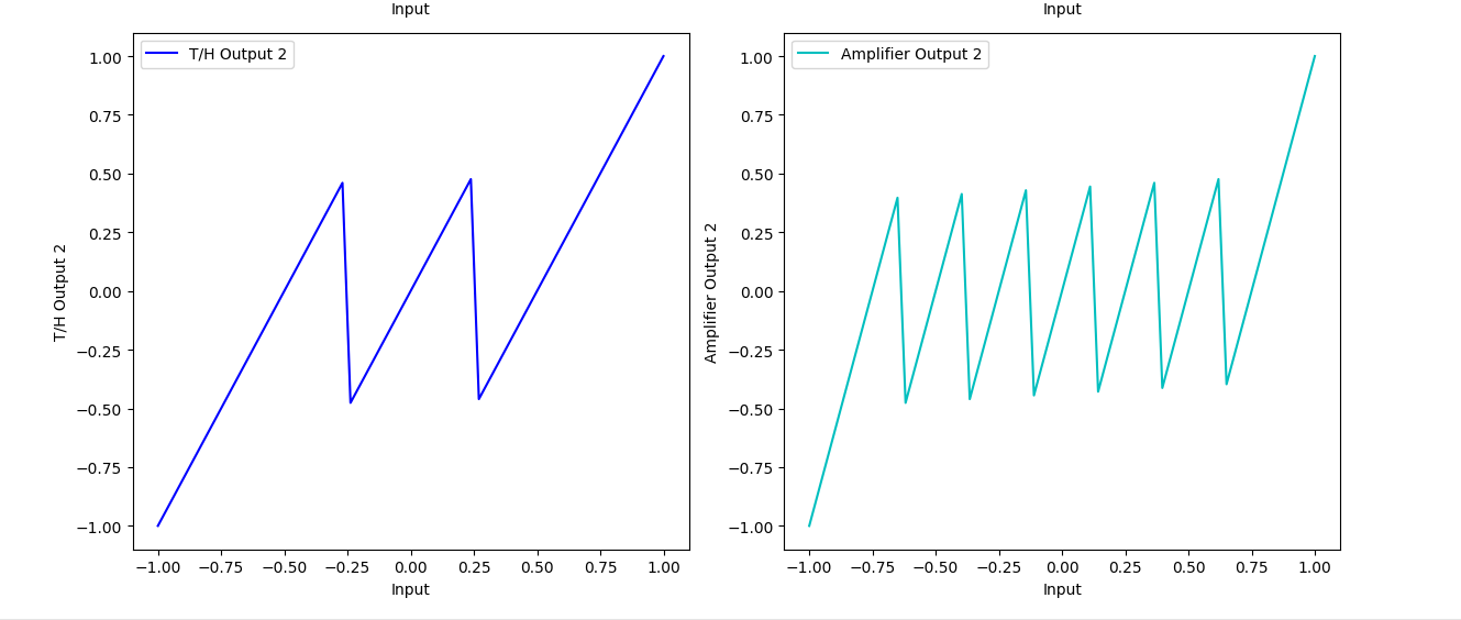
plt.plot(input_signal, th_output2, label='T/H Output 2', color='b')
plt.xlabel('Input')
plt.ylabel('T/H Output 2')
plt.legend()

plt.subplot(3, 2, 6)
plt.plot(input_signal, amp_output2, label='Amplifier Output 2', color='c')
plt.xlabel('Input')
plt.ylabel('Amplifier Output 2')
plt.legend()

plt.tight_layout()
plt.show()

import numpy as np
import pandas as pd
import matplotlib.pyplot as plt

# Number of divisions
n = 64

# Generate input signal (range from -1 to 1)
input_signal = np.linspace(-1, 1, n)

# T/H circuit output (same as input)
th_output1 = input_signal

# ADC output with special thresholds
def adc_output(th_output):
    return np.where(th_output <= -0.25, "00", 
                    np.where(th_output < 0.25, "01", "10"))

adc_output1 = adc_output(th_output1)

# DAC output based on ADC output
def dac_output(adc_output):
    return np.where(adc_output == "00", -0.5, 
                    np.where(adc_output == "01", 0, 0.5))

dac_output1 = dac_output(adc_output1)

# Subtractor output
subtractor_output1 = th_output1 - dac_output1

# 2x amplifier output
amp_output1 = subtractor_output1 * 2

# Create a DataFrame to hold all values for easy viewing
df = pd.DataFrame({
    'Input': input_signal,
    'TH Output 1': th_output1,
    'ADC Output 1': adc_output1,
    'DAC Output 1': dac_output1,
    'Subtractor Output 1': subtractor_output1,
    'Amplifier Output 1': amp_output1
})

# Print the DataFrame
print(df)

# Plotting the results
plt.figure(figsize=(12, 8))

plt.subplot(2, 2, 1)
plt.plot(input_signal, th_output1, label='T/H Output 1')
plt.xlabel('Input')
plt.ylabel('T/H Output 1')
plt.legend()

plt.subplot(2, 2, 2)
plt.plot(input_signal, dac_output1, label='DAC Output 1', color='r')
plt.xlabel('Input')
plt.ylabel('DAC Output 1')
plt.legend()

plt.subplot(2, 2, 3)
plt.plot(input_signal, subtractor_output1, label='Subtractor Output 1', color='g')
plt.xlabel('Input')
plt.ylabel('Subtractor Output 1')
plt.legend()

plt.subplot(2, 2, 4)
plt.plot(input_signal, amp_output1, label='Amplifier Output 1', color='m')
plt.xlabel('Input')
plt.ylabel('Amplifier Output 1')
plt.legend()

plt.tight_layout()
plt.show()

ランプ波

import numpy as np
import matplotlib.pyplot as plt

# Time parameters
T = 10  # total time in seconds
num_points = 1000  # number of points in the time array

# Create the time array
t = np.linspace(0, T, num_points)

# Ramp signal
V0 = np.linspace(0, 5, num_points)

# Reference voltage
VREF = 5

# Digital values
digital_values = np.zeros(num_points)

# Calculate digital values based on input voltage ranges
for i, V in enumerate(V0):
    if V < 3 * VREF / 8:
        digital_values[i] = 0  # Digital value 00
    elif 3 * VREF / 8 <= V < 4 * VREF / 8:
        digital_values[i] = 1  # Digital value 01
    elif 4 * VREF / 8 <= V < 5 * VREF / 8:
        digital_values[i] = 2  # Digital value 10
    else:
        digital_values[i] = 3  # Digital value 11

# Create labels for the digital values
digital_labels = {0: '00', 1: '01', 2: '10', 3: '11'}

# Plotting
fig, ax1 = plt.subplots()

color = 'tab:red'
ax1.set_xlabel('Time (s)')
ax1.set_ylabel('V0', color=color)
ax1.plot(t, V0, color=color)
ax1.tick_params(axis='y', labelcolor=color)

ax2 = ax1.twinx()
color = 'tab:blue'
ax2.set_ylabel('Digital Value', color=color)
ax2.plot(t, digital_values, color=color, linestyle='dashed')
ax2.tick_params(axis='y', labelcolor=color)

# Adding digital labels on the graph
for dv in np.unique(digital_values):
    idx = np.where(digital_values == dv)[0]
    ax2.fill_between(t[idx], digital_values[idx], color='tab:blue', alpha=0.1)
    ax2.text(t[idx[len(idx)//2]], dv, digital_labels[dv], color='tab:blue', 
             ha='center', va='bottom', fontsize=10, bbox=dict(facecolor='white', alpha=0.5, edgecolor='none'))

fig.tight_layout()
plt.title('Ramp Signal and Digital Values')
plt.show()

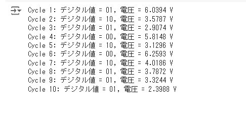
V0 = 5.14467652  # 初期入力電圧
VREF = 8.5  # 基準電圧（適切に設定してください）

# サイクル数
N = 10

# サイクルごとのデジタル値と電圧を計算
def calculate_voltage(V0, VREF, N):
    V = V0
    results = []

    for i in range(1, N + 1):
        if 0 < V < (3 * VREF / 8):
            digital_value = '00'
            V = 2 * V
        elif (3 * VREF / 8) <= V < (5 * VREF / 8):
            digital_value = '01'
            V = 2 * V - (VREF / 2)
        elif (5 * VREF / 8) <= V:
            digital_value = '10'
            V = 2 * V - VREF

        results.append((i, digital_value, V))

    return results

# 計算結果を取得
results = calculate_voltage(V0, VREF, N)

# 結果を出力
for cycle, digital_value, voltage in results:
    print(f"Cycle {cycle}: デジタル値 = {digital_value}, 電圧 = {voltage:.4f} V")

import numpy as np
import matplotlib.pyplot as plt

# Define periods
period1 = 10
period2 = period1 / 2
period3 = period1 / 4
period4 = period1 / 8

# Time axis (from 0 to period1 with step 0.001)
t = np.arange(0, period1, 0.001)

# Calculate clock signals (invert by using 1 - clk)
clk1 = 1 - (np.mod(t, period1) < period1 / 2).astype(int)
clk2 = 1 - (np.mod(t, period2) < period2 / 2).astype(int)
clk3 = 1 - (np.mod(t, period3) < period3 / 2).astype(int)
clk4 = 1 - (np.mod(t, period4) < period4 / 2).astype(int)

# Plot each clock signal separately
plt.figure(figsize=(10, 12))

# Clock 1 plot
plt.subplot(4, 1, 1)
plt.plot(t, clk1)
plt.title('Clock 1')
plt.xlabel('Time')
plt.ylabel('Signal State')
plt.ylim(-0.1, 1.1)
plt.grid(True)

# Clock 2 plot
plt.subplot(4, 1, 2)
plt.plot(t, clk2)
plt.title('Clock 2')
plt.xlabel('Time')
plt.ylabel('Signal State')
plt.ylim(-0.1, 1.1)
plt.grid(True)

# Clock 3 plot
plt.subplot(4, 1, 3)
plt.plot(t, clk3)
plt.title('Clock 3')
plt.xlabel('Time')
plt.ylabel('Signal State')
plt.ylim(-0.1, 1.1)
plt.grid(True)

# Clock 4 plot
plt.subplot(4, 1, 4)
plt.plot(t, clk4)
plt.title('Clock 4')
plt.xlabel('Time')
plt.ylabel('Signal State')
plt.ylim(-0.1, 1.1)
plt.grid(True)

# Adjust layout
plt.tight_layout()
plt.show()

def generate_digital_values(Vin1, VREF, stop_at=50):
    digital_values = []
    
    Vin = Vin1
    
    # Initial MSB calculation
    if Vin > VREF:
        Vin_next = 2 * (Vin - VREF)
        digital_values.append(1)
    else:
        Vin_next = 2 * Vin
        digital_values.append(0)
    
    print(f"Vin1 = {Vin:.5f}, Digital Value = {digital_values[0]}")
    
    # Calculate subsequent MSBs up to stop_at
    for i in range(2, stop_at + 1):
        Vin = Vin_next
        if Vin > VREF:
            Vin_next = 2 * (Vin - VREF)
            digital_values.append(1)
        else:
            Vin_next = 2 * Vin
            digital_values.append(0)
        
        print(f"Vin{i} = {Vin:.5f}, Digital Value = {digital_values[-1]}")
    
    return digital_values

# Example usage:
VREF = 10.0
Vin1 = 3.77777

print(f"Reference Voltage (VREF) = {VREF} V")
print(f"Input Voltage (Vin1) = {Vin1} V")

digital_values = generate_digital_values(Vin1, VREF, stop_at=50)