CMOSアナログ/ディジタルIC設計の基礎: CMOS回路はSPICEを使ってトランジスタでこうつくる (半導体シリーズ) Pythonコード

P20~23
ID=IDsat×(1+λVDS)

IDsat=(1/2)μ×Cox×(W/L)(VGS-Vth)^2

VGS=√(ID/((1/2)×μ×Cox×(W/L)))+Vth

import math

def calculate_IDsat(mu, Cox, W, L, VGS, Vth):
    return 0.5 * mu * Cox * (W / L) * (VGS - Vth)**2

def calculate_ID(mu, Cox, W, L, IDsat, lambda_VDS):
    return IDsat * (1 + lambda_VDS)

def calculate_VGS(ID, mu, Cox, W, L, Vth):
    return math.sqrt(ID / (0.5 * mu * Cox * (W / L))) + Vth

# Parameters (example values)
mu = 200e-6  # Mobility in cm^2/(V·s)
Cox = 1e-8   # Oxide capacitance per unit area in F/cm^2
W = 10e-6    # Width in meters
L = 1e-6     # Length in meters
Vth = 1      # Threshold voltage in volts
lambda_VDS = 0.02  # Channel-length modulation parameter

# Example VGS value
VGS = 1.8  # Gate-source voltage in volts

# Calculations
IDsat = calculate_IDsat(mu, Cox, W, L, VGS, Vth)
ID = calculate_ID(mu, Cox, W, L, IDsat, lambda_VDS)
calculated_VGS = calculate_VGS(ID, mu, Cox, W, L, Vth)

# Output the results
print(f"IDsat: {IDsat} A")
print(f"ID: {ID} A")
print(f"Calculated VGS: {calculated_VGS} V")

P30
I=VDD/R1-VOUT/R1
横軸VOUT 縦軸I

import numpy as np
import matplotlib.pyplot as plt

# Define the parameters
VDD = 5.0  # Supply voltage in volts
R1 = 1e3  # Resistance in ohms

# Define the range for VOUT
VOUT = np.linspace(0, VDD, 500)  # 500 points from 0 to VDD

# Calculate the current I
I = (VDD - VOUT) / R1

# Plot the results
plt.figure(figsize=(10, 6))
plt.plot(VOUT, I, label='Current I vs VOUT', color='blue')
plt.xlabel('VOUT (V)')
plt.ylabel('I (A)')
plt.title('Current I vs VOUT')
plt.grid(True)
plt.legend()
plt.show()

P107
gm1=μ×Cox×(W/L)(VGS-Vth)
gm2=√(2× μ×Cox×(W/L)× IDsat)
IDsat=(1/2)μ×Cox×(W/L)(VGS-Vth)^2

import math

# Constants and parameters
mu = 1e-4  # Mobility (example value)
Cox = 1e-8  # Oxide capacitance per unit area (example value)
W = 1e-6  # Width of the MOSFET (example value)
L = 1e-6  # Length of the MOSFET (example value)
VGS = 1.0  # Gate-source voltage (example value)
Vth = 0.2  # Threshold voltage (example value)

# Calculate gm1
gm1 = mu * Cox * (W / L) * (VGS - Vth)

# Calculate IDsat
IDsat = 0.5 * mu * Cox * (W / L) * (VGS - Vth) ** 2

# Calculate gm2
gm2 = math.sqrt(2 * mu * Cox * (W / L) * IDsat)

# Display the results
print(f"gm1 = {gm1:.3e} S")
print(f"gm2 = {gm2:.3e} S")
print(f"IDsat = {IDsat:.3e} A")

P109負荷アンプ回路
-gm×(出力抵抗1×出力抵抗2)/(出力抵抗1+出力抵抗2)

import numpy as np

# Define the parameters
gm = 1e-1  # Transconductance in Siemens
R1 = 1   # Output resistance 1 in ohms
R2 = 2e10   # Output resistance 2 in ohms

# Calculate the gain
gain = -gm * (R1 * R2) / (R1 + R2)

# Convert the gain to decibels (dB)
gain_dB = 20 * np.log10(abs(gain))

# Display the results
print(f"Gain: {gain}")
print(f"Gain in dB: {gain_dB}")

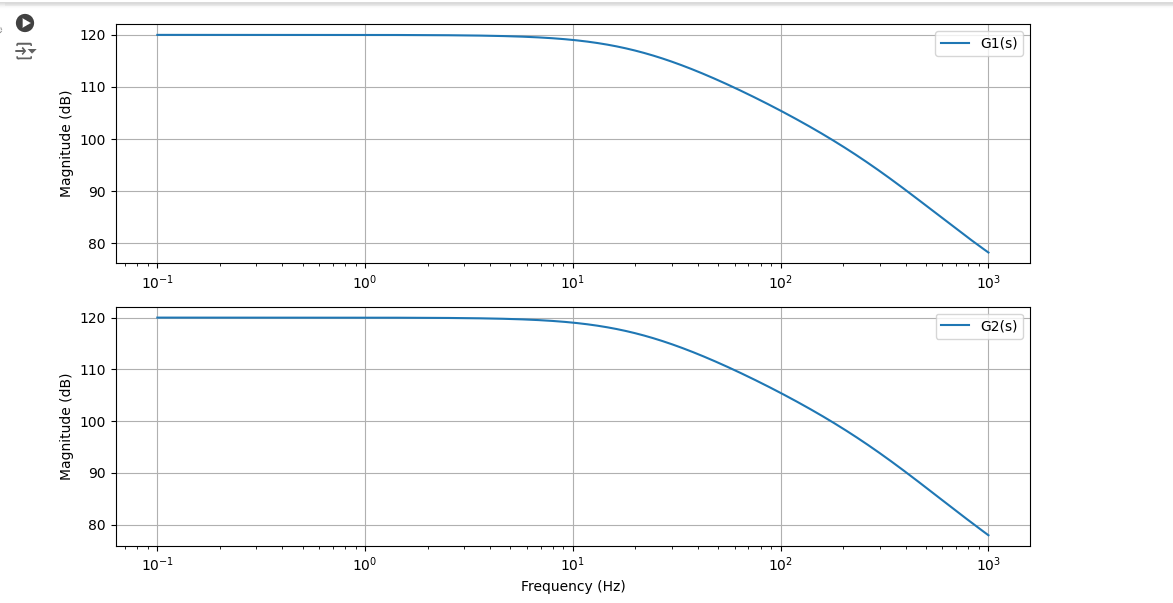
P121
2段増幅CMOSアンプ位相補償回路

import numpy as np
import matplotlib.pyplot as plt
from scipy import signal

# Given parameters (example values, replace with actual values)
gm1 = 35e-6  # Given in micro (μ)
gm6 = 23e-6  # Given in micro (μ)
R1 = 50e6    # Given in ohms
R2 = 25e6    # Given in ohms
Cc = 1       # Replace with actual value if different
Rc = 1       # Replace with actual value if different

# Frequencies (in rad/s)
wp1 = 2 * np.pi * 2.88
wp2 = 2 * np.pi * 1.8e6
wp3 = 2 * np.pi * 965e3
wzA = 2 * np.pi * 2.8
wzB = 2 * np.pi * 22e6

# Transfer functions G1 and G2
num1 = [-wzA, 1]  # Numerator of G1
den = np.polymul([1/wp1, 1], np.polymul([1/wp2, 1], [1/wp3, 1]))  # Denominator common for both
num2 = [1/wzB, 1]  # Numerator of G2

# Construct transfer functions
G1 = signal.TransferFunction(num1, den)
G2 = signal.TransferFunction(num2, den)

# Frequency range for Bode plot
w = np.logspace(0, 8, 1000)

# Calculate the product gm1 * gm6 * R1 * R2
product = gm1 * gm6 * R1 * R2

# Convert product to decibels
product_db = 20 * np.log10(product)
print(f"The product gm1 * gm6 * R1 * R2 is: {product:.4e}")
print(f"The product in dB is: {product_db:.2f} dB")

# Bode plot for G1 and G2 combined
plt.figure(figsize=(10, 8))

# Bode plot for G1
plt.subplot(2, 1, 1)
w, mag1, phase1 = signal.bode(G1, w)
plt.semilogx(w, mag1, label='G1')
plt.title('Bode plots of G1(s) and G2(s)')
plt.ylabel('Magnitude (dB)')
plt.grid(which='both', axis='both')
plt.legend()

plt.subplot(2, 1, 2)
plt.semilogx(w, phase1)
plt.ylabel('Phase (degrees)')
plt.xlabel('Frequency (rad/s)')
plt.grid(which='both', axis='both')

# Bode plot for G2
plt.subplot(2, 1, 1)
w, mag2, phase2 = signal.bode(G2, w)
plt.semilogx(w, mag2, label='G2')
plt.ylabel('Magnitude (dB)')
plt.grid(which='both', axis='both')
plt.legend()

plt.subplot(2, 1, 2)
plt.semilogx(w, phase2)
plt.ylabel('Phase (degrees)')
plt.xlabel('Frequency (rad/s)')
plt.grid(which='both', axis='both')

plt.tight_layout()
plt.show()

import numpy as np
import matplotlib.pyplot as plt

# Define the parameters
B = 1000
C = 20
D = 300
E = 4000

# Define the transfer functions G1(s) and G2(s)
def G1(s, A):
    return A * (1 - s/B) / ((1 + s/C) * (1 + s/D))

def G2(s, A):
    return A * (1 + s/B) / ((1 + s/C) * (1 + s/D) * (1 + s/E))

# Calculate Bode magnitude in dB for G1(s) and G2(s)
def calculate_bode_plot(A_G1, A_G2):
    omega = np.logspace(-1, 3, 1000)
    s = 1j * omega

    mag_G1 = 20 * np.log10(np.abs(G1(s, A_G1)))
    mag_G2 = 20 * np.log10(np.abs(G2(s, A_G2)))

    return omega, mag_G1, mag_G2

# Plot Bode plots for G1(s) and G2(s)
def plot_bode(A_G1, A_G2):
    omega, mag_G1, mag_G2 = calculate_bode_plot(A_G1, A_G2)

    plt.figure(figsize=(10, 6))

    # Bode plot for G1(s)
    plt.subplot(2, 1, 1)
    plt.semilogx(omega, mag_G1, label='G1(s)')
    plt.ylabel('Magnitude (dB)')
    plt.grid(True)
    plt.legend()

    # Bode plot for G2(s)
    plt.subplot(2, 1, 2)
    plt.semilogx(omega, mag_G2, label='G2(s)')
    plt.xlabel('Frequency (Hz)')
    plt.ylabel('Magnitude (dB)')
    plt.grid(True)
    plt.legend()

    plt.tight_layout()
    plt.show()

# Set the value of A
A_G1 = 1000000
A_G2 = 1000000

# Run the plotting function
plot_bode(A_G1, A_G2)

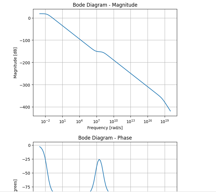
P１２３

import numpy as np
import matplotlib.pyplot as plt
from scipy import signal

# Given values
A1 = 2000000000
A2 = 6000000000
Cc = 2e-12  # Capacitance in farads (2 pico farads)
C1 = 184e-15  # Capacitance in farads (184 femto farads)
C2 = 239e-15  # Capacitance in farads (239 femto farads)
RC = 70e3  # Resistance in ohms (70 kilo ohms)
rop2 = 8e3  # Resistance in ohms (8 kilo ohms)
ron4 = 8e3  # Resistance in ohms (8 kilo ohms)
rop6 = 8e3  # Resistance in ohms (8 kilo ohms)
ron7 = 8e3  # Resistance in ohms (8 kilo ohms)

# Compute intermediate values
R1 = (rop2 * ron4) / (rop2 + ron4)
R2 = (rop6 * ron7) / (rop6 + ron7)
A = A1 * A2
gm1 = A1 / R1
gm6 = A2 / R2
a = gm6 * Cc * R1 * R2
b = (C1 + C2) / gm6
h = (C1 * C2 * RC) / (C1 + C2)
B = Cc * (RC - (1 / gm6))

# Display computed values
print(f"C1 (Parasitic Capacitance): {C1} F")
print(f"C2 (Parasitic Capacitance): {C2} F")
print(f"R1: {R1} Ohms")
print(f"R2: {R2} Ohms")
print(f"A: {A} (Linear), {20 * np.log10(A)} dB")
print(f"gm1: {gm1} S")
print(f"gm6: {gm6} S")
print(f"a: {a}")
print(f"b: {b}")
print(f"h: {h}")
print(f"B: {B}")

# Define the transfer function
num = [A, A / B]  # Numerator coefficients
den = np.convolve([1, 1/a], np.convolve([1, 1/b], [1, 1/h]))  # Denominator coefficients

# Create the transfer function system
system = signal.TransferFunction(num, den)

# Generate Bode plot
w, mag, phase = signal.bode(system)

# Plot magnitude
plt.figure()
plt.semilogx(w, mag)
plt.title('Bode Diagram - Magnitude')
plt.xlabel('Frequency [rad/s]')
plt.ylabel('Magnitude [dB]')
plt.grid()

# Plot phase
plt.figure()
plt.semilogx(w, phase)
plt.title('Bode Diagram - Phase')
plt.xlabel('Frequency [rad/s]')
plt.ylabel('Phase [degrees]')
plt.grid()

plt.show()