Pythonで理解する電気回路

メモ代わりに使っていきます。

https://www2-kawakami.ct.osakafu-u.ac.jp/lecture/
キャパシタとコイルの式

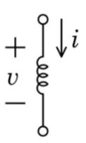
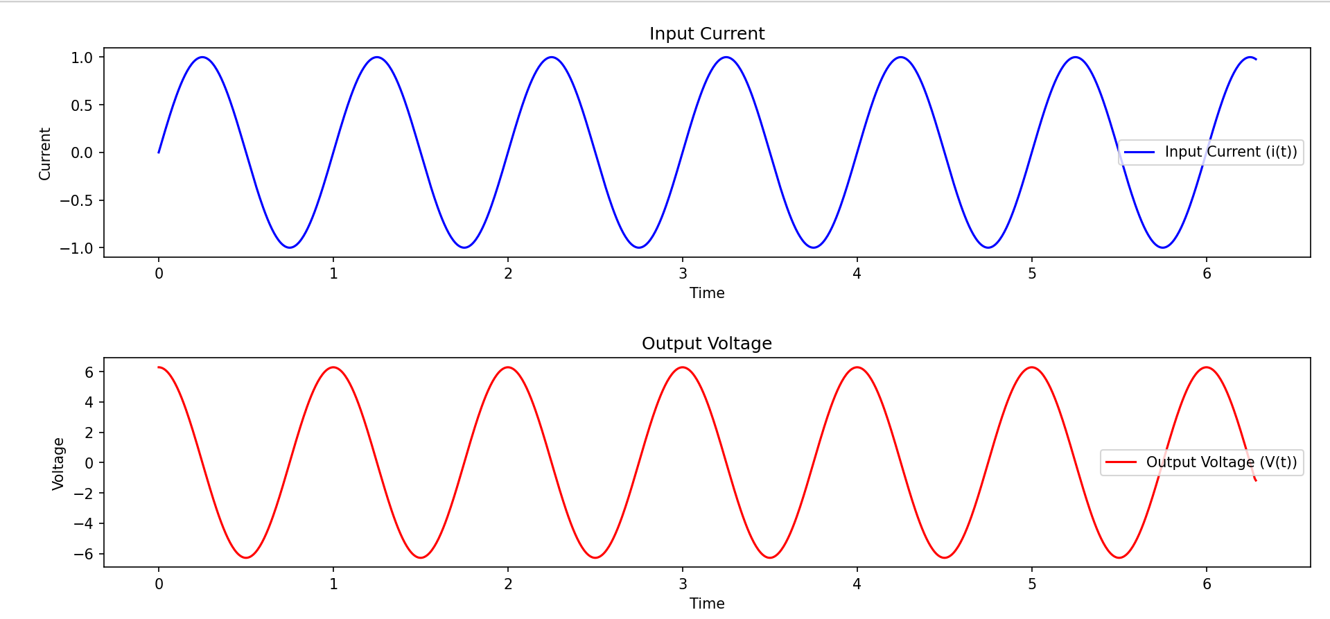
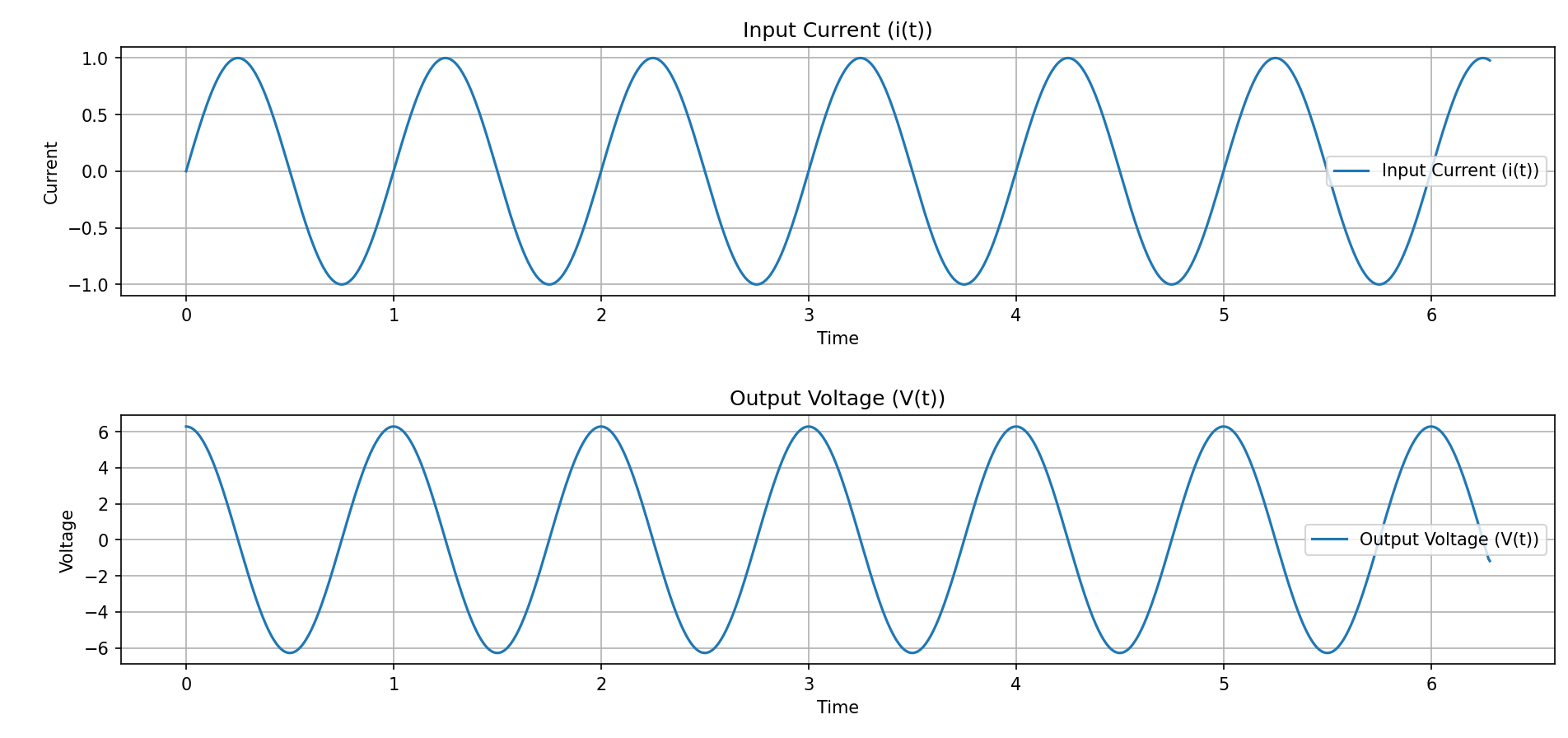
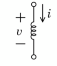
コイルの式
L’i(t)=V(t)
電流(t)をtで微分した後にLをかけるとV(t)となる

import numpy as np
import matplotlib.pyplot as plt

# 定数定義
ω = 2*np.pi  # 角周波数
L = 1        # インダクタンス

# 時間の範囲を定義
t = np.linspace(0, 2*np.pi, 1000)

# 入力電流
i_t = np.sin(ω*t)

# 出力電圧
V_t = L * np.gradient(i_t, t)

# プロット
plt.figure(figsize=(10, 5))

plt.subplot(2, 1, 1)
plt.plot(t, i_t, label='Input Current (i(t))', color='blue')
plt.xlabel('Time')
plt.ylabel('Current')
plt.title('Input Current')
plt.legend()

plt.subplot(2, 1, 2)
plt.plot(t, V_t, label='Output Voltage (V(t))', color='red')
plt.xlabel('Time')
plt.ylabel('Voltage')
plt.title('Output Voltage')
plt.legend()

plt.tight_layout()
plt.show()

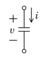
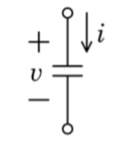
キャパシタの式
CV’(t)=I(t)
電圧(t)をtで微分した後にCをかけるとI(t)となる

import numpy as np
import matplotlib.pyplot as plt

# パラメータ
C = 1e-6  # キャパシタンス（1μF）
L = 1     # インダクタンス（1H）
omega = 2*np.pi  # 角周波数

# 時間配列
t = np.linspace(0, 2*np.pi, 1000)

# 入力電流
i_t = np.sin(omega * t)

# 出力電圧
V_t = L * np.gradient(i_t, t)

# プロット
plt.figure(figsize=(10, 5))

plt.subplot(2, 1, 1)
plt.plot(t, i_t, label='Input Current (i(t))')
plt.xlabel('Time')
plt.ylabel('Current')
plt.title('Input Current (i(t))')
plt.grid(True)
plt.legend()

plt.subplot(2, 1, 2)
plt.plot(t, V_t, label='Output Voltage (V(t))')
plt.xlabel('Time')
plt.ylabel('Voltage')
plt.title('Output Voltage (V(t))')
plt.grid(True)
plt.legend()

plt.tight_layout()
plt.show()

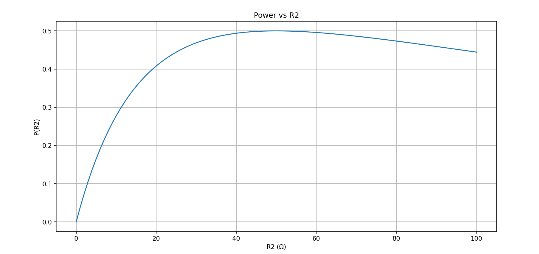
P(R2)=((V/(R1+R2))^2)×R2
R1を入力側抵抗、R2を出力側抵抗
R1=50Ω

import numpy as np
import matplotlib.pyplot as plt

# Given values
R1 = 50  # 入力側抵抗

# 関数定義
def calculate_P_R2(V, R2):
    return ((V / (R1 + R2)) ** 2) * R2

# パラメータ設定
V = 10  # 仮の電圧

# R2の値を範囲内で変化させる
R2_values = np.linspace(0, 100, 100)  # 範囲は必要に応じて変更可能

# P(R2)を計算
P_R2_values = calculate_P_R2(V, R2_values)

# プロット
plt.plot(R2_values, P_R2_values)
plt.xlabel('R2 (Ω)')
plt.ylabel('P(R2)')
plt.title('Power vs R2')
plt.grid(True)
plt.show()

import numpy as np

# 与えられた値
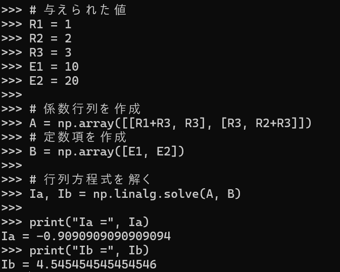
R1 = 1
R2 = 2
R3 = 3
E1 = 10
E2 = 20

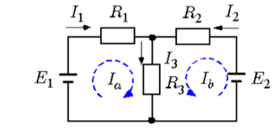
# 係数行列を作成
A = np.array([[R1+R3, R3], [R3, R2+R3]])
# 定数項を作成
B = np.array([E1, E2])

# 行列方程式を解く
Ia, Ib = np.linalg.solve(A, B)

print("Ia =", Ia)
print("Ib =", Ib)

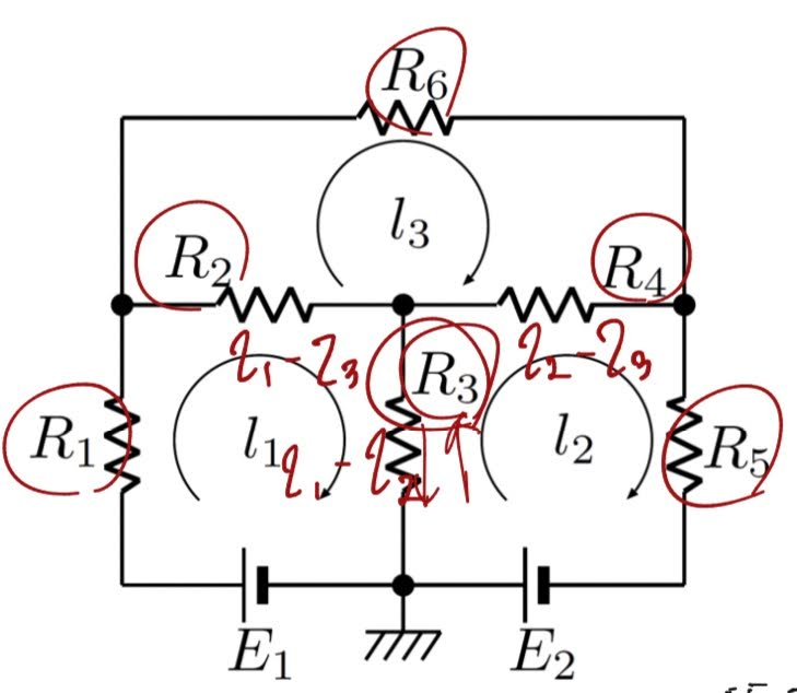
import numpy as np

# 係数行列 A を定義
A = np.array([[R1 + R2 + R3, -R3, -R2],
              [-R3, R3 + R4 + R5, -R4],
              [-R2, -R4, R2 + R4 + R6]])

# 右辺のベクトル b を定義
b = np.array([E1, E2, 0])

# 逆行列を計算
A_inv = np.linalg.inv(A)

# 解を計算
x = np.dot(A_inv, b)

# 解を表示
print("解 (i1, i2, i3):", x)

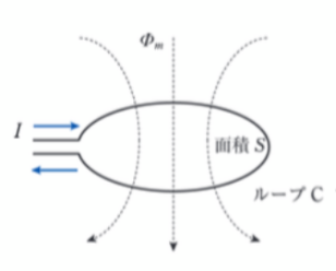
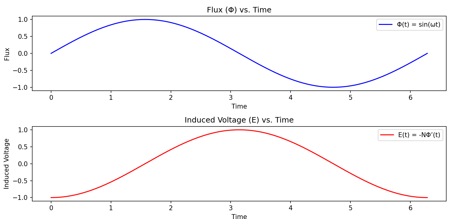
import numpy as np
import matplotlib.pyplot as plt

# パラメータの設定
N = 1  # 巻数
omega = 1  # 角周波数

# 時間の範囲を設定
t = np.linspace(0, 2*np.pi, 1000)

# 磁束と起電力の計算
flux = np.sin(omega * t)
induced_voltage = -N * omega * np.cos(omega * t)

# プロット
plt.figure(figsize=(10, 5))

# 磁束のプロット
plt.subplot(2, 1, 1)
plt.plot(t, flux, label='Φ(t) = sin(ωt)', color='blue')
plt.title('Flux (Φ) vs. Time')
plt.xlabel('Time')
plt.ylabel('Flux')
plt.legend()

# 起電力のプロット
plt.subplot(2, 1, 2)
plt.plot(t, induced_voltage, label='E(t) = -NΦ’(t)', color='red')
plt.title('Induced Voltage (E) vs. Time')
plt.xlabel('Time')
plt.ylabel('Induced Voltage')
plt.legend()

plt.tight_layout()
plt.show()

共振

import numpy as np

# インピーダンスの計算
def calculate_impedance(R, L, C, omega):
    XL = omega * L  # インダクタンスのリアクタンス
    XC = 1 / (omega * C)  # キャパシタンスのリアクタンス
    impedance = np.sqrt(R**2 + (XL - XC)**2)
    return impedance

# 共振周波数の計算
def calculate_resonant_frequency(L, C):
    return 1 / (2 * np.pi * np.sqrt(L * C))

# Qの計算
def calculate_quality_factor(L, C, resonant_frequency, bandwidth):
    return resonant_frequency / bandwidth

# パラメータの設定
R = 100  # 抵抗（単位: オーム）
L = 0.1  # インダクタンス（単位: ヘンリー）
C = 1e-6  # キャパシタンス（単位: ファラド）
omega = 2 * np.pi * 1000  # 角周波数（単位: ラジアン/秒）
bandwidth = 1000  # 帯域幅（単位: Hz）

# インピーダンスの計算
impedance = calculate_impedance(R, L, C, omega)
print("Impedance:", impedance, "ohms")

# 共振周波数の計算
resonant_frequency = calculate_resonant_frequency(L, C)
print("Resonant Frequency:", resonant_frequency, "Hz")

# Qの計算
quality_factor = calculate_quality_factor(L, C, resonant_frequency, bandwidth)
print("Quality Factor:", quality_factor)

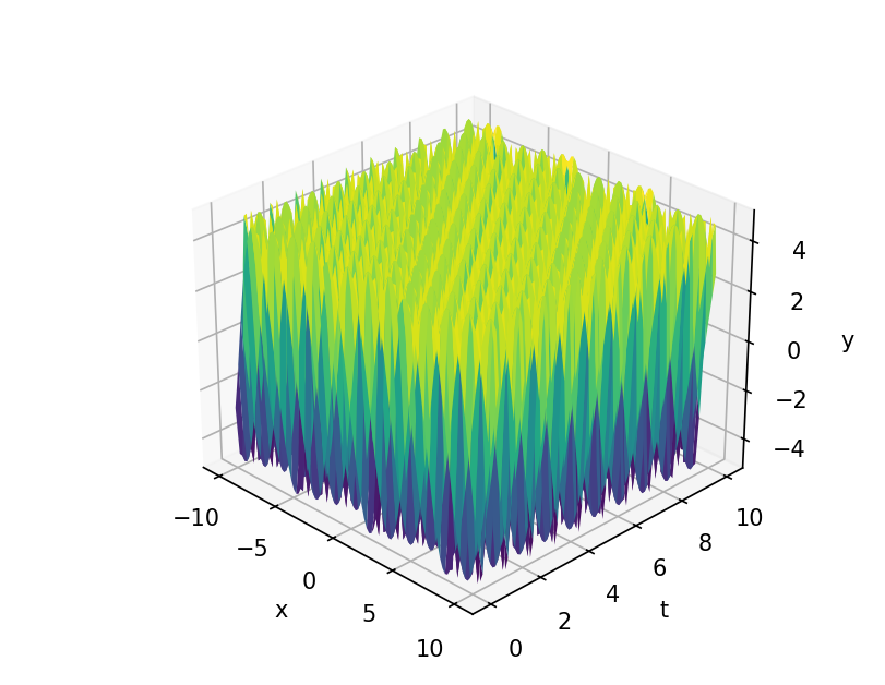
波

import numpy as np
import matplotlib.pyplot as plt
from mpl_toolkits.mplot3d import Axes3D

# 定数の設定
A = 5  # 振幅
T = 1  # 時間周期
w = 2 * np.pi / T  # 角周波数
lmbda = 1  # 波長

# 空間と時間の範囲を設定
x = np.linspace(-10, 10, 100)
t = np.linspace(0, 10, 100)

# 空間と時間の格子を生成
X, T = np.meshgrid(x, t)

# 波動関数の計算
Y = A * np.sin(w * T - (X / lmbda))

# 三次元プロット
fig = plt.figure()
ax = fig.add_subplot(111, projection='3d')
ax.plot_surface(X, T, Y, cmap='viridis')

# 軸ラベルの設定
ax.set_xlabel('x')
ax.set_ylabel('t')
ax.set_zlabel('y')

# グラフを表示
plt.show()

import numpy as np
import matplotlib.pyplot as plt
from mpl_toolkits.mplot3d import Axes3D

def y(t, theta, A, omega):
    return A * np.sin(omega * t + theta)

# tとθの範囲を設定
t = np.linspace(0, 10, 100)  # tの範囲と点の数を設定
theta = np.linspace(0, 2 * np.pi, 100)  # θの範囲と点の数を設定
T, Theta = np.meshgrid(t, theta)  # 2次元のメッシュグリッドを作成

# 振幅と角周波数を設定
A = 1
omega = 1

# yの値を計算
Y = y(T, Theta, A, omega)

# 3Dプロット
fig = plt.figure()
ax = fig.add_subplot(111, projection='3d')
ax.plot_surface(T, Theta, Y, cmap='viridis')

# 軸ラベル
ax.set_xlabel('t')
ax.set_ylabel('θ')
ax.set_zlabel('y')

import numpy as np
import matplotlib.pyplot as plt

# ωの値を設定します
ω = 2 * np.pi

# tの範囲を設定します
t = np.linspace(0, 2*np.pi, 1000)

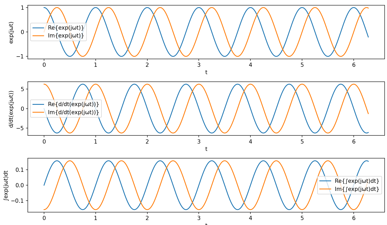
# exp(jωt)とその微分、積分を計算します
exp_jωt = np.exp(1j * ω * t)
diff_exp_jωt = 1j * ω * exp_jωt
int_exp_jωt = (1 / (1j * ω)) * exp_jωt

# プロットします
plt.figure(figsize=(10, 6))

plt.subplot(3, 1, 1)
plt.plot(t, np.real(exp_jωt), label='Re{exp(jωt)}')
plt.plot(t, np.imag(exp_jωt), label='Im{exp(jωt)}')
plt.xlabel('t')
plt.ylabel('exp(jωt)')
plt.legend()

plt.subplot(3, 1, 2)
plt.plot(t, np.real(diff_exp_jωt), label='Re{d/dt(exp(jωt))}')
plt.plot(t, np.imag(diff_exp_jωt), label='Im{d/dt(exp(jωt))}')
plt.xlabel('t')
plt.ylabel('d/dt(exp(jωt))')
plt.legend()

plt.subplot(3, 1, 3)
plt.plot(t, np.real(int_exp_jωt), label='Re{∫exp(jωt)dt}')
plt.plot(t, np.imag(int_exp_jωt), label='Im{∫exp(jωt)dt}')
plt.xlabel('t')
plt.ylabel('∫exp(jωt)dt')
plt.legend()

plt.tight_layout()
plt.show()

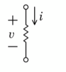
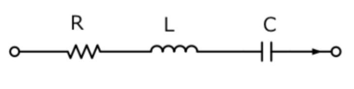
i(s)×R=V(s)
i(s)×(sL)=V(s)
i(s)×(1/(sC))=V(s)

伝達関数について、抵抗はR、コイルは(sL)、キャパシタは(1/(Cs))とする

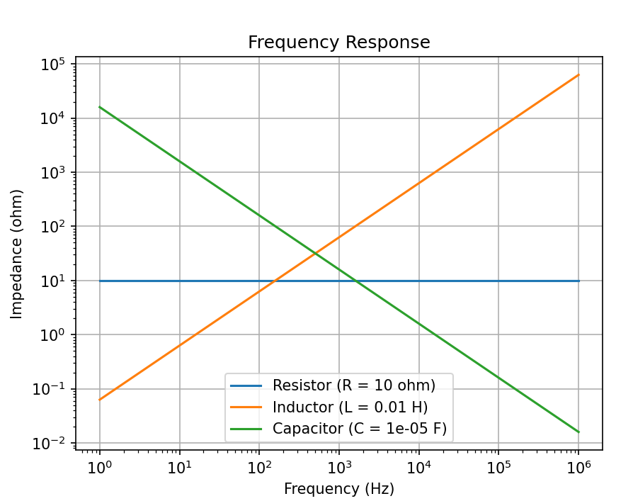
抵抗はRとコイルは(sL)とキャパシタは(1/(Cs))で周波数応答をみる

ボード線図

import numpy as np
import matplotlib.pyplot as plt

# 抵抗の周波数応答
def resistor_response(freq, R):
    return np.ones_like(freq) * R

# コイルの周波数応答
def inductor_response(freq, L):
    return 1j * 2 * np.pi * freq * L

# キャパシタの周波数応答
def capacitor_response(freq, C):
    return 1 / (1j * 2 * np.pi * freq * C)

# 周波数範囲の設定
freq = np.logspace(0, 6, 1000)  # 1 Hz から 1 MHz まで

# 抵抗の周波数応答をプロット
R = 10  # 抵抗値
resistor_impedance = resistor_response(freq, R)
plt.loglog(freq, np.abs(resistor_impedance), label='Resistor (R = {} ohm)'.format(R))

# コイルの周波数応答をプロット
L = 0.01  # ヘンリー（H）
inductor_impedance = inductor_response(freq, L)
plt.loglog(freq, np.abs(inductor_impedance), label='Inductor (L = {} H)'.format(L))

# キャパシタの周波数応答をプロット
C = 0.00001  # ファラド（F）
capacitor_impedance = capacitor_response(freq, C)
plt.loglog(freq, np.abs(capacitor_impedance), label='Capacitor (C = {} F)'.format(C))

# プロットの設定
plt.xlabel('Frequency (Hz)')
plt.ylabel('Impedance (ohm)')
plt.title('Frequency Response')
plt.legend()
plt.grid(True)
plt.show()

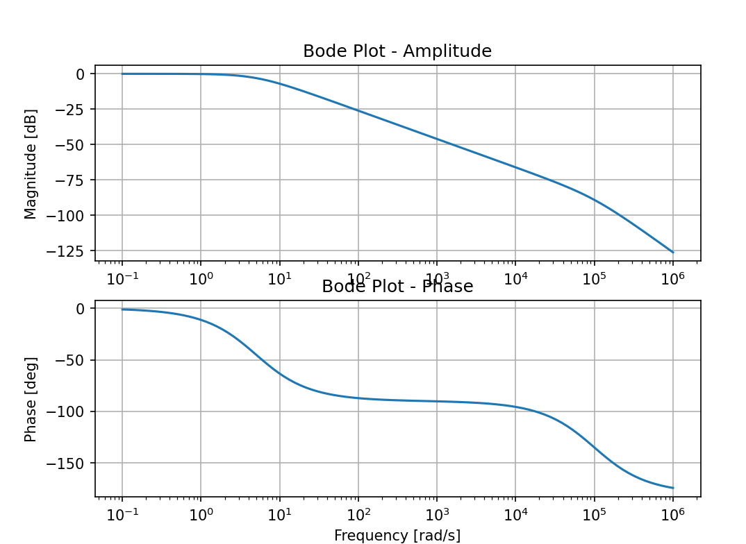
RCL直列回路

import numpy as np
import matplotlib.pyplot as plt
from scipy import signal

# 伝達関数の係数を定義
R = 1
L = 0.2  # Lの値を変更
C = 0.00001  # Cの値を変更
s = signal.TransferFunction([1], [C*L, R*L, 1])

# 周波数応答を計算
w, mag, phase = signal.bode(s)

# Bodeプロットを描画
plt.figure()
plt.subplot(2, 1, 1)
plt.semilogx(w, mag)  # 振幅プロット
plt.title('Bode Plot - Amplitude')
plt.ylabel('Magnitude [dB]')
plt.grid(True)

plt.subplot(2, 1, 2)
plt.semilogx(w, phase)  # 位相プロット
plt.title('Bode Plot - Phase')
plt.xlabel('Frequency [rad/s]')
plt.ylabel('Phase [deg]')
plt.grid(True)
plt.show()

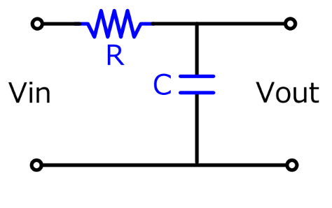
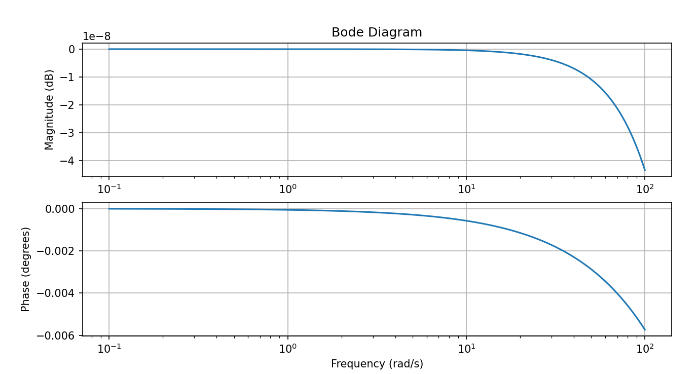
RC積分回路
伝達関数=(1/(sC))/(R+1/(sC))

import numpy as np
import matplotlib.pyplot as plt

# パラメータの設定
R = 1
C = 0.000001

# 角周波数の範囲を設定
omega = np.logspace(-1, 2, 400)

# 伝達関数の計算
s = 1j * omega
H = (1/(s*C)) / (R + 1/(s*C))

# 大きさと位相の計算
magnitude = np.abs(H)
phase = np.angle(H, deg=True)

# ボード線図のプロット
plt.figure(figsize=(10, 5))
plt.subplot(2, 1, 1)
plt.semilogx(omega, 20 * np.log10(magnitude))
plt.title('Bode Diagram')
plt.ylabel('Magnitude (dB)')
plt.grid(True)

plt.subplot(2, 1, 2)
plt.semilogx(omega, phase)
plt.xlabel('Frequency (rad/s)')
plt.ylabel('Phase (degrees)')
plt.grid(True)

plt.show()

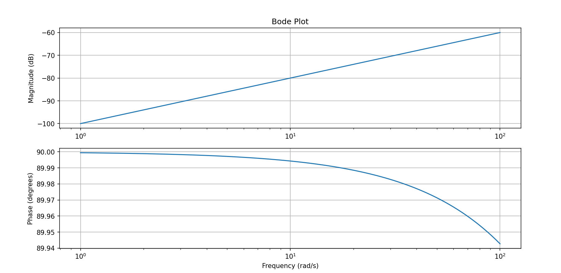
CR微分回路
伝達関数=(R)/(R+1/(sC))
https://t-design-free.com/cr-circuit/

import numpy as np
import matplotlib.pyplot as plt

# 伝達関数の定義
R = 1
C = 0.00001
def transfer_function(omega):
    s = 1j * omega
    return R / (R + 1 / (s * C))

# 大きさと位相を計算する関数
def magnitude_phase(omega):
    tf = transfer_function(omega)
    magnitude = np.abs(tf)
    phase = np.angle(tf, deg=True) # 引数deg=Trueで位相を度数法で取得
    return magnitude, phase

# 周波数の範囲を設定
omega = np.logspace(0, 2, 100) # 1から100までの対数スケールの周波数配列

# 大きさと位相の配列を計算
magnitude, phase = magnitude_phase(omega)

# ボード線図をプロット
plt.figure(figsize=(10, 6))

plt.subplot(2, 1, 1)
plt.semilogx(omega, 20 * np.log10(magnitude))
plt.title('Bode Plot')
plt.ylabel('Magnitude (dB)')
plt.grid()

plt.subplot(2, 1, 2)
plt.semilogx(omega, phase)
plt.xlabel('Frequency (rad/s)')
plt.ylabel('Phase (degrees)')
plt.grid()

plt.show()

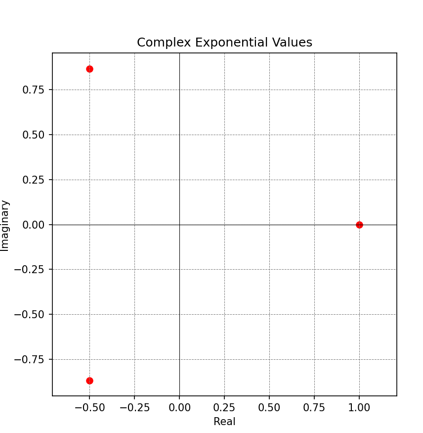
ベクトルオペレーター
https://jeea.or.jp/course/contents/01153/

import numpy as np
import matplotlib.pyplot as plt

# 角度（ラジアン）を定義
angles = np.array([2*np.pi/3, 4*np.pi/3, 6*np.pi/3])

# 指数関数を計算
exponential_values = np.exp(1j * angles)

# 実部と虚部を取得
real_part = np.real(exponential_values)
imaginary_part = np.imag(exponential_values)

# プロット
plt.figure(figsize=(6, 6))
plt.scatter(real_part, imaginary_part, color='red')
plt.axhline(0, color='black',linewidth=0.5)
plt.axvline(0, color='black',linewidth=0.5)
plt.grid(color = 'gray', linestyle = '--', linewidth = 0.5)
plt.xlabel('Real')
plt.ylabel('Imaginary')
plt.title('Complex Exponential Values')
plt.axis('equal')
plt.show()

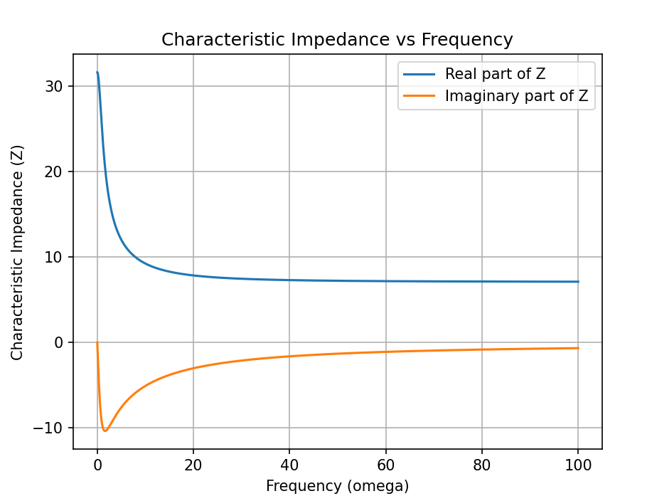
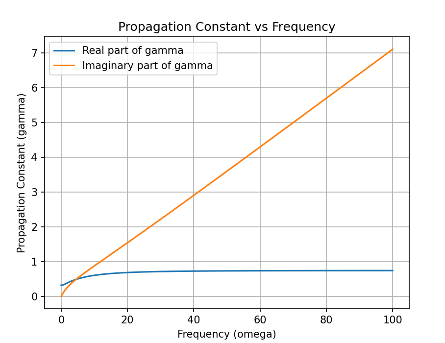
分布定数回路
http://asaseno.aki.gs/tech/bunpu01.html

伝搬定数

import numpy as np
import matplotlib.pyplot as plt

# 定義されていない変数を設定
R = 10
L = 0.5
G = 0.01
C = 0.01
omega = np.linspace(0, 100, 1000)  # 0から100までの1000点でomegaを定義

# gammaとZの計算
gamma = np.sqrt((R + 1j * omega * L) * (G + 1j * omega * C))
Z = np.sqrt((R + 1j * omega * L) / (G + 1j * omega * C))

# プロット
plt.figure()
plt.plot(omega, np.real(gamma), label='Real part of gamma')
plt.plot(omega, np.imag(gamma), label='Imaginary part of gamma')
plt.xlabel('Frequency (omega)')
plt.ylabel('Propagation Constant (gamma)')
plt.legend()
plt.title('Propagation Constant vs Frequency')
plt.grid(True)

plt.figure()
plt.plot(omega, np.real(Z), label='Real part of Z')
plt.plot(omega, np.imag(Z), label='Imaginary part of Z')
plt.xlabel('Frequency (omega)')
plt.ylabel('Characteristic Impedance (Z)')
plt.legend()
plt.title('Characteristic Impedance vs Frequency')
plt.grid(True)

plt.show()