離散差分方程式の描写

import numpy as np
import matplotlib.pyplot as plt

# フィルターのパラメータ
T = 1.0  # サンプリング周期
C = 1.0  # 容量
R = 1.0  # 抵抗

# フィルター係数の計算
T1 = T / (C * R)

# ローパスフィルターの係数
a_lp = 1 / (1 + T1)
b_lp = T1 / (1 + T1)

# ハイパスフィルターの係数
b_hp = 1 - T1

# 周波数レンジ
frequencies = np.logspace(-1, 2, 400)  # 0.1Hzから100Hzまでの範囲
omega = 2 * np.pi * frequencies * T

# 周波数応答の計算
H_lp = (a_lp + b_lp * np.exp(-1j * omega)) / (1 - b_lp * np.exp(-1j * omega))
H_hp = (1 - np.exp(-1j * omega) + b_hp * np.exp(-1j * omega)) / (1 - b_hp * np.exp(-1j * omega))

# プロット
plt.figure(figsize=(12, 6))

# ローパスフィルターの周波数応答
plt.subplot(1, 2, 1)
plt.title('Low-Pass Filter Frequency Response')
plt.semilogx(frequencies, 20 * np.log10(np.abs(H_lp)))
plt.xlabel('Frequency [Hz]')
plt.ylabel('Magnitude [dB]')
plt.grid(which='both', linestyle='--', linewidth=0.5)

# ハイパスフィルターの周波数応答
plt.subplot(1, 2, 2)
plt.title('High-Pass Filter Frequency Response')
plt.semilogx(frequencies, 20 * np.log10(np.abs(H_hp)))
plt.xlabel('Frequency [Hz]')
plt.ylabel('Magnitude [dB]')
plt.grid(which='both', linestyle='--', linewidth=0.5)

plt.tight_layout()
plt.show()

import numpy as np
import matplotlib.pyplot as plt

# パラメータの定義
L = 1.0  # インダクタンス (H)
R = 1.0  # 抵抗 (Ohm)
T = 0.01  # サンプリング周期 (s)
E = 1.0  # 定電圧 (V)
time_duration = 1.0  # シミュレーション時間 (s)

# 時間のベクトル
t = np.arange(0, time_duration, T)
N = len(t)

# 電流のベクトル
i = np.zeros(N)

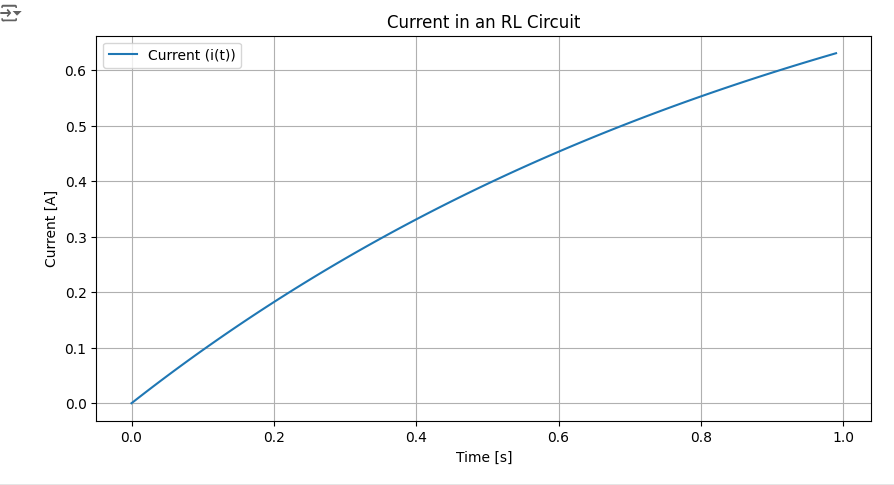
# オイラー法で微分方程式を解く
for k in range(1, N):
    di = (T / L) * (E - R * i[k-1])
    i[k] = i[k-1] + di

# プロット
plt.figure(figsize=(10, 5))
plt.plot(t, i, label='Current (i(t))')
plt.title('Current in an RL Circuit')
plt.xlabel('Time [s]')
plt.ylabel('Current [A]')
plt.grid()
plt.legend()
plt.show()

import numpy as np
import matplotlib.pyplot as plt

def low_pass_filter_continuous(K, T, u, t):
    """連続時間ローパスフィルターのシミュレーション"""
    dt = t[1] - t[0]
    y = np.zeros_like(u)
    x = np.zeros_like(u)
    for i in range(1, len(t)):
        dx = (1/T) * (K * u[i] - x[i-1])
        x[i] = x[i-1] + dx * dt
        y[i] = x[i]
    return y

def low_pass_filter_discrete(K, T, Ts, u):
    """離散時間ローパスフィルターのシミュレーション"""
    y = np.zeros_like(u)
    x = np.zeros_like(u)
    alpha = Ts / T
    for n in range(1, len(u)):
        x[n] = (1 - alpha) * x[n-1] + K * alpha * u[n]
        y[n] = x[n]
    return y

# パラメータの定義
K = 1.0  # フィルターのゲイン
T = 0.1  # フィルターの時定数
Ts = 0.01  # サンプリング時間
t = np.arange(0, 1, Ts)  # シミュレーション時間
u = np.sin(2 * np.pi * 5 * t)  # 入力信号 (5Hzのサイン波)

# 連続時間フィルターのシミュレーション
y_cont = low_pass_filter_continuous(K, T, u, t)

# 離散時間フィルターのシミュレーション
y_disc = low_pass_filter_discrete(K, T, Ts, u)

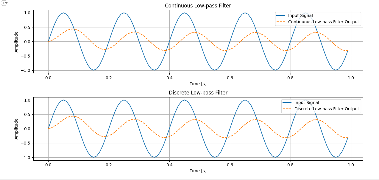
# プロット
plt.figure(figsize=(12, 6))

plt.subplot(2, 1, 1)
plt.plot(t, u, label='Input Signal')
plt.plot(t, y_cont, label='Continuous Low-pass Filter Output', linestyle='--')
plt.title('Continuous Low-pass Filter')
plt.xlabel('Time [s]')
plt.ylabel('Amplitude')
plt.legend()
plt.grid()

plt.subplot(2, 1, 2)
plt.plot(t, u, label='Input Signal')
plt.plot(t, y_disc, label='Discrete Low-pass Filter Output', linestyle='--')
plt.title('Discrete Low-pass Filter')
plt.xlabel('Time [s]')
plt.ylabel('Amplitude')
plt.legend()
plt.grid()

plt.tight_layout()
plt.show()

import numpy as np
import matplotlib.pyplot as plt

# Parameters
T = 0.1  # Sampling period
t = np.arange(0, 10, T)  # Time vector

# Analog sine signal
A = np.sin(2 * np.pi * t)

# C is the same as A (A + B = C)
C = A

# B is C delayed by period T
B = np.roll(C, int(T / (t[1] - t[0])))

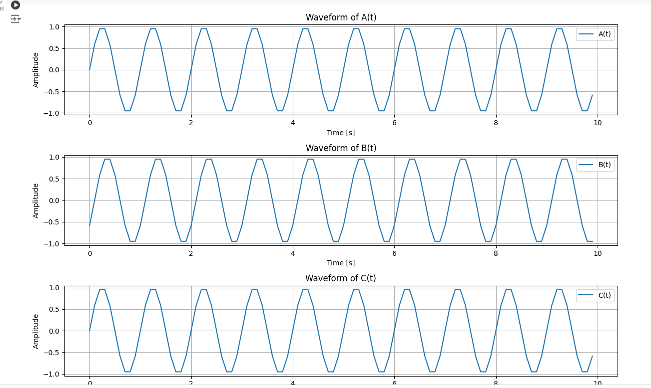
# Plot the waveforms separately
plt.figure(figsize=(12, 8))

# Plot A(t)
plt.subplot(3, 1, 1)
plt.plot(t, A, label='A(t)')
plt.xlabel('Time [s]')
plt.ylabel('Amplitude')
plt.title('Waveform of A(t)')
plt.legend()
plt.grid(True)

# Plot B(t)
plt.subplot(3, 1, 2)
plt.plot(t, B, label='B(t)')
plt.xlabel('Time [s]')
plt.ylabel('Amplitude')
plt.title('Waveform of B(t)')
plt.legend()
plt.grid(True)

# Plot C(t)
plt.subplot(3, 1, 3)
plt.plot(t, C, label='C(t)')
plt.xlabel('Time [s]')
plt.ylabel('Amplitude')
plt.title('Waveform of C(t)')
plt.legend()
plt.grid(True)

plt.tight_layout()
plt.show()

import numpy as np
import matplotlib.pyplot as plt

# Parameters
T = 0.1  # Sampling period
t = np.arange(0, 10, T)  # Time vector

# Analog sine signal
A = np.sin(2 * np.pi * t)

# B is the same as A (A + C = B)
B = A

# C is B delayed by period T
C = np.roll(B, int(T / (t[1] - t[0])))

# Plot the waveforms separately
plt.figure(figsize=(12, 8))

# Plot A(t)
plt.subplot(3, 1, 1)
plt.plot(t, A, label='A(t)')
plt.xlabel('Time [s]')
plt.ylabel('Amplitude')
plt.title('Waveform of A(t)')
plt.legend()
plt.grid(True)

# Plot B(t)
plt.subplot(3, 1, 2)
plt.plot(t, B, label='B(t)')
plt.xlabel('Time [s]')
plt.ylabel('Amplitude')
plt.title('Waveform of B(t)')
plt.legend()
plt.grid(True)

# Plot C(t)
plt.subplot(3, 1, 3)
plt.plot(t, C, label='C(t)')
plt.xlabel('Time [s]')
plt.ylabel('Amplitude')
plt.title('Waveform of C(t)')
plt.legend()
plt.grid(True)

plt.tight_layout()
plt.show()