Gradient Descent - Beginner's Guide

Introduction.

When starting machine learning in university, one of the firstly learn a thing is a gradient descent. Gradient descent is a viral optimization algorithm utilized to train machine learning.
It is used in neural network modeling to achieve better results by returning the most minor possible error.

I'm not going to theory part in this article. Let's see how it works using PyTorch.

gd.py

import torch
import matplotlib.pyplot as plt
torch.manual_seed(1989);

First, let's generate values for the x-axis.
We can utilize torch.arrange(start,end) function.

gd.py

X = torch.arange(0,15).float()
X

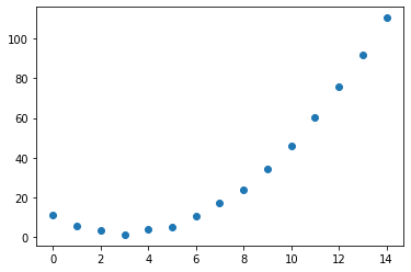
Now it's time to generate data for the Y-axis. I will use the quadratic function here, and it is better to make some noise, so it will bit closer to actual data.

gd.py

Y = torch.rand(15)*3 +0.9*(X-3)**2+1
plt.scatter(X,Y);

Now we need to find a function that agrees with our data points. It is like a quadratic function (Please act like we didn't use a quadratic function to generate the data. LOL)
The generic equation for a quadratic function is ax²+bx+c

gd.py

def func(x,params):
  a, b, c = params
  return a*(x**2)+(b*x)+c

Mean squared error (MSE) will be used for the loss function. MSE is calculated by taking the average squared of difference between the predicted value and actual value.

gd.py

def mse(preds, actual): 
    return ((preds-actual)**2).mean()

For the next step, we need to know about the learning rate. Since we are not focusing on the theory part, I'm not going to describe it. Definition for the learning rate is step size for updating the parameter for each iteration while minimizing the loss. If the step size is bigger, it can be faster vice versa if the step size is small, it will be slow. And also, there are some issues related to diverging and etc. Usually, we can start from a small value.

Now, let's generated 3 random values for parameters, and we need to track the gradient. In PyTorch, we can easily track it by using requires_grad_() .
Then we can set the learning rate, and also we need to copy the initial parameter values that we need to use for the later part.

gd.py

params = torch.randn(3).requires_grad_()
print(params)
original_params = params.clone()
lr = 1e-4

Now let's create a function to visualize the predicted and actual data.

gd.py

def show_plot(preds, ax=None):
    if ax is None: ax=plt.subplots()[1]
    ax.scatter(X, Y)
    ax.scatter(X, preds.detach().numpy(), color='red')
    ax.set_ylim(-75,120)

Model

1) Init the weights.
2) Calculate loss.
3) Utilizing parameters.required_grads_ of PyTorch permits, calling backward on loss and then assisting in calculating the parameters' gradient.
4) Calculate the parameters' gradient by multiplying it with the learning rate and subtracting it from the original parameters.
5) Reset parameter's gradients.
6) Print RMSE.
7) Return prediction.

gd.py

def step(params):
  preds= func(X, params)
  loss = mse(preds, Y)
  loss.backward()
  params.data = params.data - lr*params.grad.data
  params.grad = None
  print("RMSE:",(loss.item())**0.5)
  return preds

Then it's time to run the model for 10 iterations and how it behaves.

gd.py

_,axs = plt.subplots(1,10,figsize=(15,3))
for ax in axs: show_plot(step(params), ax)
plt.tight_layout()

By checking the RMSE, we can see the error is getting lower for each iteration. And from the graph, we can see that first, the red dots are much different from the blue dots, which means there is a significant difference between the actual and predicted values. But with the increase of iterations, the deviation between actual and predicted values getting lower.

Let's run another 10 iterations.

gd.py

_,axs = plt.subplots(1,10,figsize=(15,3))
for ax in axs: show_plot(step(params), ax)
plt.tight_layout()

Again, we can see that the error is getting lower, and predicted values are trying to be set on the actual values with the iterations.

In this article, we have studied how Gradient decent works in deep learning. let us meet again with another ML article.

*本記事は @qualitia_cdevの中の一人、@nuwanさんが書いてくれました。
*This article is written by @nuwan a member of @qualitia_cdev.