オイラー法と中心差分法とルンゲクッタ法で、以下の常微分方程式の解を計算する。
\frac{dx}{dt}=f(t)=cos(t)
一般解
\begin{eqnarray}
dx&=&cos(t)dt\\
\int{dx}&=&\int{cos(t)}dt\\
x&=&sin(t)+x(t=0)
\end{eqnarray}
オイラー法
$x(t+Δt)$をテイラー展開すると、
x(t+Δt)=x(t)+\frac{dx(t)}{dt}Δt+O(Δt^2)
$O(Δt^2)$を打ち切り誤差として切り捨てると
\begin{eqnarray}
x(t+Δt)&≃&x(t)+\frac{dx(t)}{dt}Δt\\
&=&x(t)+cos(t)Δt...①
\end{eqnarray}
となり、$t+Δt$での$x$を$t$での$x$を用いて逐次計算していく方法。
アルゴリズムは
- $t、x$に初期値を与える。
- ①式により$t+Δt$での$x$を求める。
- 計算したい範囲2を繰り返す。
・ソースコード
import math
import matplotlib.pyplot as plt
import numpy as np

def f(t):
    return math.cos(t)

DELTA_T = 0.001
MAX_T = 100.0

t = 0.0 # t初期値
x = 0.0 # t=0でのx

x_hist = [x]
t_hist = [t]

# 逐次計算
while t < MAX_T:
    x += f(t)*DELTA_T
    t += DELTA_T
    x_hist.append(x)
    t_hist.append(t)

# 数値解のプロット
plt.plot(t_hist, x_hist)

# 厳密解(sin(t))のプロット
t = np.linspace(0, MAX_T, 1/DELTA_T)
x = np.sin(t)
plt.plot(t, x)

plt.xlim(0, MAX_T)
plt.ylim(-1.3, 1.3)

plt.show()
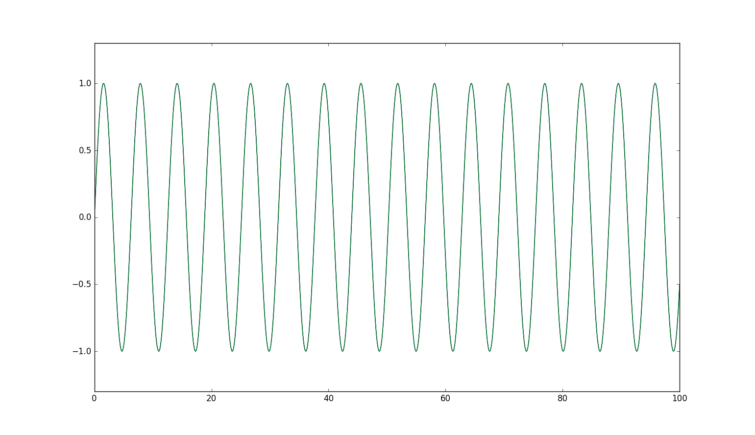
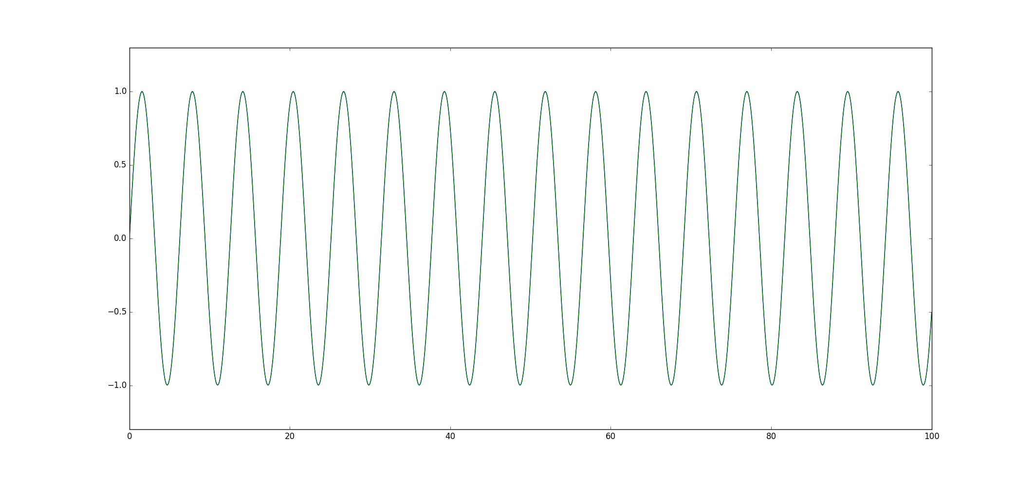
・結果
Δt=0.01
Δt=0.001
中心差分法
$x(t+Δt)$、$x(t-Δt)$をテイラー展開すると、
\begin{eqnarray}
x(t+Δt)&=&x(t)+\frac{dx(t)}{dt}Δt+\frac{1}{2}\frac{d^2x}{dt^2}Δt^2+O(Δt^3)...①\\
x(t-Δt)&=&x(t)-\frac{dx(t)}{dt}Δt+\frac{1}{2}\frac{d^2x}{dt^2}Δt^2+O(Δt^3)...②
\end{eqnarray}
①-②し、$O(Δt^3)$を切り捨てると
\begin{eqnarray}
x(t+Δt)-x(t-Δt)&≃&2\frac{dx(t)}{dt}Δt\\
x(t+Δt)&≃&x(t-Δt)+2cos(t)Δt...③\\
\end{eqnarray}
$t+Δt$⇒$t$で置き換えると
\begin{eqnarray}
x(t)&≃&x(t-2Δt)+2cos(t-Δt)Δt...③\\
\end{eqnarray}
$t-2Δt$での$x$がわかっているとき、③式により$t$での$x$を逐次的に計算していく方法。
・ソースコード
import math
import matplotlib.pyplot as plt
import numpy as np

def f(t):
    return math.cos(t)

DELTA_T = 0.001
MAX_T = 100.0

t = 0.0 # t初期値
x = 0.0 # t=0でのx

x_hist = [x]
t_hist = [t]

while t < MAX_T:
    x += 2*f(t-DELTA_T)*DELTA_T
    t += 2*DELTA_T
    x_hist.append(x)
    t_hist.append(t)

# 数値解のプロット
plt.plot(t_hist, x_hist)

# 厳密解(sin(t))のプロット
t = np.linspace(0, MAX_T, 1/DELTA_T)
x = np.sin(t)
plt.plot(t, x)

plt.xlim(0, MAX_T)
plt.ylim(-1.3, 1.3)

plt.show()
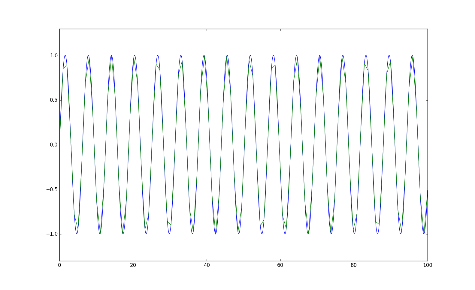
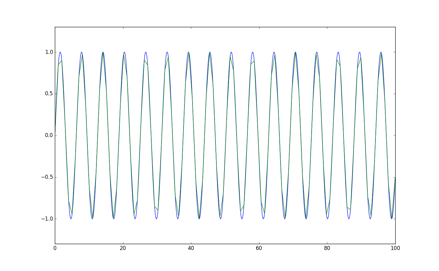
・結果
$Δt=0.01$
$Δt=0.001$
4次ルンゲクッタ法
\begin{eqnarray}
k_1&=&Δtf(t,x)\\
k_2&=&Δtf(t+\frac{Δt}{2}, x(t)+\frac{k_1}{2})\\
k_3&=&Δtf(t+\frac{Δt}{2}, x(t)+\frac{k_2}{2})\\
k_4&=&Δtf(t+Δt, x(t)+k_3)\\
x(t+Δt)&=&x(t)+\frac{1}{6}(k_1+2k_2+2k_3+k_4)
\end{eqnarray}
により、$t+Δt$での$x$を、$t$での$x$を用いて逐次的に計算していく方法。
$f(t,x)=f(t)$のときは、$k_2=k_3$より
\begin{eqnarray}
x(t+Δt)&=&x(t)+\frac{1}{6}(k_1+4k_2+k_4)
\end{eqnarray}
$x(t+Δt)$に含まれる誤差は$O(Δt^5)$
・ソースコード
import math
import matplotlib.pyplot as plt
import numpy as np

def f(t):
    return math.cos(t)

DELTA_T = 0.001
MAX_T = 100.0

t = 0.0 # t初期値
x = 0.0 # t=0でのx

x_hist = [x]
t_hist = [t]

# 逐次計算
while t < MAX_T:
    k1 = DELTA_T*f(t)
    k2 = DELTA_T*f(t+DELTA_T/2)
    k3 = DELTA_T*f(t+DELTA_T/2)
    k4 = DELTA_T*f(t+DELTA_T)
    x += (k1 + 2*k2 + 2*k3 + k4)/6
    t += DELTA_T
    x_hist.append(x)
    t_hist.append(t)

# 数値解のプロット
plt.plot(t_hist, x_hist)

# 厳密解(sin(t))のプロット
t = np.linspace(0, MAX_T, 1/DELTA_T)
x = np.sin(t)
plt.plot(t, x)

plt.xlim(0, MAX_T)
plt.ylim(-1.3, 1.3)

plt.show()
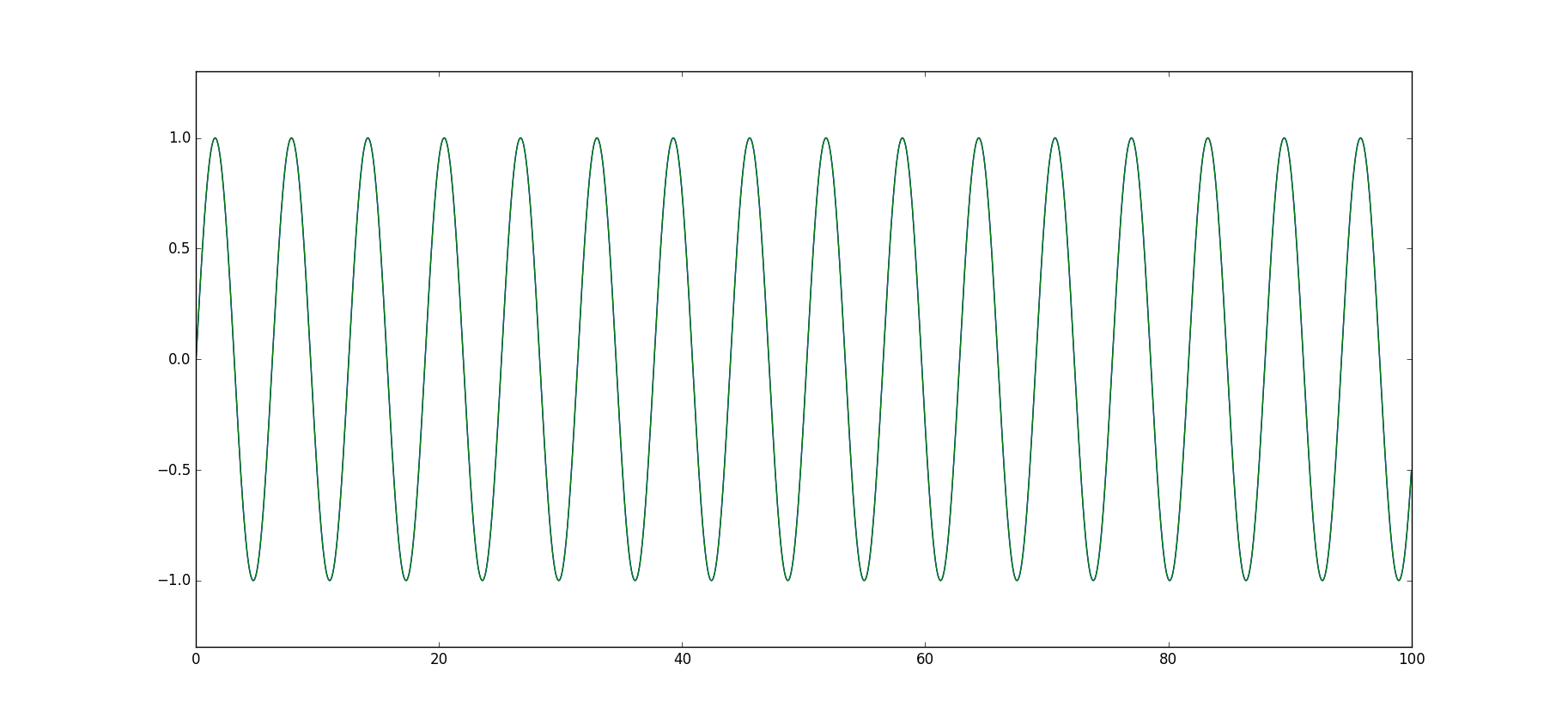
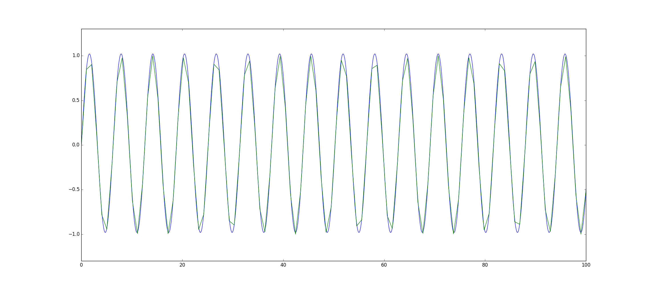
・結果
$Δt=0.001$
$Δt=0.001$