More than 1 year has passed since last update.

[Pythonによる物理シミュレーション] 万有引力を受ける天体の軌道。1中心1体系、ルンゲクッタ法

Last updated at 2021-12-10Posted at 2021-12-09

2021/12/9 投稿

0.メニュー

1.問題設定
2.運動方程式の数値解法
3.計算コード
4.可視化、アニメーション

万有引力を受ける物体の運動方程式を数値的に解き、下図のように天体の運動をシミュレートしていきます。

1.問題設定

運動方程式

\vec{r}(t) := (x(t),y(t))  \tag{1.1}

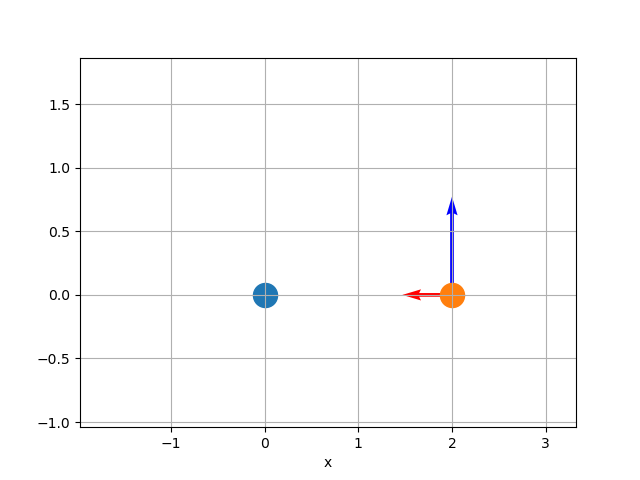
質量$m$のオレンジ色の天体が質量$M$の青い天体から万有引力を受けながら運動している。この時オレンジ色の天体が受ける力(赤いベクトル)を数式で表すと


\vec{f} = -\frac{GMm}{|\vec{r}|^2} \frac{\vec{r}}{|\vec{r}|}
\tag{1.2}

向きが位置ベクトル$\vec{r}$の反対方向になっている
この問題に対する運動方程式は

m \frac{d^2 \vec{r}(t)}{dt^2} = -\frac{GMm}{|\vec{r}|^2} \frac{\vec{r}}{|\vec{r}|}
\tag{1.3}

初期条件

図のようにx軸上に配置し、y軸方向に初速を与えるから

\vec{r}(t=0) = (R_0, 0) \space\space\space\space
\vec{v}(t=0) = (0, v_{y0})
\tag{1.4, 1.5}

等速円運動する条件

やみくもに初速を与えるとスイングバイして飛びだしてしまい物理的に面白い解が得られないので、式$(1.5)$の$v_{y0}$を等速円運動する条件を基準に決める。円運動するときの初速を$v_0$とすると

m \frac{v_0^2}{R_0} = \frac{GMm}{R_0^2}
\tag{1.6}

上の式は高校物理でも出てくる式です。式$(1.6)$を変形すると

v_0 = \sqrt{\frac{GM}{R_0}}
\tag{1.7}

式$(1.7)$を基準に$v_{y0}$を決める。$v_{y0}=v_0$とき式$(1.3)$を解くと円運動するような解が得られる。

2.運動方程式の数値解法

連立1階微分方程式

式$(1.3)$を4次ルンゲッタ法を用いて解く。そのために1階微分方程式に書き直す

\frac{d \vec{r}}{dt} = \vec{v}
\space\space\space\space\space\space
\frac{d \vec{v}}{dt} = -\frac{GM}{|\vec{r}|^2} \frac{\vec{r}}{|\vec{r}|} 
\tag{2.1, 2.2}

プログラム上で取り扱いやすくするため、変数を行列形式にまとめる

\textbf{X}(t) := \begin{pmatrix} \vec{r} & \vec{v} \end{pmatrix} = 
\begin{pmatrix}
x & v_x \\
y & v_y
\end{pmatrix}
\tag{2.3}

\textbf{F}(\textbf{X}(t)) :=
\begin{pmatrix} \vec{v} & -GM \cdot \vec{r}/|\vec{r}|^3 \end{pmatrix} 
= 
\begin{pmatrix}
v_x & -GM \cdot x/|\vec{r}|^3 \\
v_y & -GM \cdot y/|\vec{r}|^3
\end{pmatrix}
\tag{2.4}

したがって式$(2.1),(2.2)$も以下のように書き換えられる

\frac{d \textbf{X}(t)}{dt} = \textbf{F}(\textbf{X}(t))
\tag{2.5}

ルンゲクッタ法

(\Delta_1, \Delta_2, \Delta_3, \Delta_4) :=(0, \Delta t /2, \Delta t /2, \Delta t)
\tag{2.6}

(\beta_1, \beta_2, \beta_3, \beta_4) :=(1, 2, 2, 1)
\tag{2.7}

\textbf{K}_0 := \textbf{O} \space\space\space\space\space\space
\textbf{K}_{i} := \textbf{F}(\textbf{X}(t) + \Delta_i \textbf{K}_{i-1})
\tag{2.8, 2.9}

\textbf{X}(t+\Delta t) = \textbf{X}(t) + \sum_{k=1}^{4} \beta_k \textbf{K}_{k}
\tag{2.10}

ただし$\textbf{O}$は零行列

\textbf{O} := \begin{pmatrix}
0 & 0 \\
0 & 0
\end{pmatrix}
\tag{2.11}

初期値$\textbf{X}(t=0)$を決めれば芋ずる式に値が求まる。

\textbf{X}(t=0) = \begin{pmatrix}
R_0 & 0 \\
0 & v_{y0}
\end{pmatrix}
\tag{2.12}

3. 計算コード


import numpy as np

# 物理定数
M_pa = 1.0 
G_pa = 1.0

# 時間変数
tmin = 0.0 
tmax = 20.0 
dt = 0.001
t = tmin

# 微分方程式の右辺  式(2.4)
def f(G, M, x_mat):
    # パラメーター
    _GM = -1.0*G*M
    # 各成分
    x = x_mat[0][0]
    y = x_mat[1][0]
    vx = x_mat[0][1]
    vy = x_mat[1][1]
    # 距離の3乗
    r3 = (x**2 + y**2)**1.5
    # 戻り値
    re = np.array([
        [vx, _GM*x/r3],
        [vy, _GM*y/r3]
    ])
    return re


# 数値解用変数
x_mat = np.zeros((2, 2))

# 初期条件
r0 = 2
# 第一宇宙速度
v0 = (G_pa*M_pa/r0)**0.5   # 式(1.7)
#
# 式(2.12)
x_mat[:, 0] = np.array([
    r0, 
    0
])
x_mat[:, 1] = np.array([
    0, 
    0.7*v0
])



# ルンゲクッタ変数
beta = [0.0, 1.0, 2.0, 2.0, 1.0]   # 式(2.6)
delta = [0.0, 0.0, dt/2, dt/2, dt]  # 式(2.7)
k_rk = np.zeros((5, 2, 2))

# データカット
sb_dt = 0.1
Nt = 1
count = 1
cat_val = int(sb_dt/dt)
x_lis = [x_mat.copy()]

# 時間積分
while t < tmax:
    sum_x = np.zeros((2, 2))
    for k in [1, 2, 3, 4]:
        k_rk[k, :, :] = f(G_pa, M_pa, x_mat + delta[k]*k_rk[k-1, :, :]) # 式(2.9)
        sum_x += beta[k]*k_rk[k, :, :] # 式(2.10)の途中計算
    #
    x_mat += (dt/6)*sum_x  # 式(2.10)
    # データカット
    if count%cat_val == 0:
        x_lis.append(x_mat.copy())
        Nt += 1
    #
    count += 1
    t += dt


# データ取得
x_t = np.array(x_lis)[:, 0, 0]
y_t = np.array(x_lis)[:, 1, 0]
vx_t = np.array(x_lis)[:, 0, 1]
vy_t = np.array(x_lis)[:, 1, 1]
xmin, xmax = x_t.min(), x_t.max()
ymin, ymax = y_t.min(), y_t.max()
width = xmax - xmin
hight = ymax - ymin

4.可視化、アニメーション

コード

import matplotlib.pyplot as plt
import matplotlib.animation as animation

fig, ax = plt.subplots()

lim_add = 0.5
vec_size = 0.2
def animate_move(i):
    plt.cla()
    plt.xlabel('x')
    plt.xlim(xmin - lim_add*width, xmax + lim_add*width)
    plt.ylim(ymin - lim_add*hight, ymax + lim_add*hight)
    plt.scatter(0, 0, s=300)
    # 距離
    r_val = (x_t[i]**2 + y_t[i]**2)**0.5
    # 動径方向の単位ベクトル
    er = np.array([x_t[i], y_t[i]])/r_val
    # 万有引力ベクトル
    m_pa = 1.0
    f_vec = -1.0*(G_pa*M_pa*m_pa/(r_val**2)) * er.copy()
    plt.quiver(x_t[i], y_t[i], f_vec[0], f_vec[1], scale=vec_size**-1, color='red')
    # 速度ベクトル
    plt.quiver(x_t[i], y_t[i], vx_t[i], vy_t[i], scale=vec_size**-1, color='blue')
    # 速度の大きさ
    v_val = (vx_t[i]**2 + vy_t[i]**2)**0.5
    # 遠心力ベクトル
    m_pa = 1.0
    f_vec = (m_pa*v_val**2)/r_val * er.copy()
    plt.quiver(x_t[i], y_t[i], f_vec[0], f_vec[1], scale=vec_size**-1, color='green')
    # 軌跡
    plt.plot(x_t[0:i], y_t[0:i], '--')
    plt.scatter(x_t[i], y_t[i], s=300)
    plt.grid()



animate = animate_move
kaisu = Nt - 1
anim = animation.FuncAnimation(fig,animate,frames=kaisu,interval=10)
anim.save("animete_1.gif", writer="imagemagick")
plt.show()