この記事では天文学でよく使われるpythonモジュールであるastropyとastroqueryを使って星座について説明ていきます。
星座の領域区分
大昔から人々は星空を見て星々を色んなグループに組んでそれは星座となった。星座の区分は人や国によって全然違うが、現在一般に使われるのは国際天文学連合によって定義された88の星座です。
天球上のすべての領域は必ず88の星座の中の一つに属します。天球上の星座の区分は地球上の国家の境界よりも簡単で、すべての境界線は赤道座標上の直線によって描かれています。
星座の区分を定義するのは4列×357行の表。詳しくはRoman et al. (1987)を。
その表はastropyのモジュールの中にも収められています。それをastropyのTableに読み込んで使えます。
import astropy.coordinates
from astropy.table import Table
import os

dat_path = os.path.join(astropy.coordinates.__path__[0],'data','constellation_data_roman87.dat')
ctable = Table.read(dat_path,format='ascii')
print(ctable)
  col1    col2    col3  col4
------- ------- ------- ----
    0.0    24.0    88.0  UMi
    8.0    14.5    86.5  UMi
   21.0    23.0 86.1667  UMi
   18.0    21.0    86.0  UMi
    0.0     8.0    85.0  Cep
 9.1667 10.6667    82.0  Cam
    0.0     5.0    80.0  Cep
10.6667    14.5    80.0  Cam
   17.5    18.0    80.0  UMi
20.1667    21.0    80.0  Dra
    ...     ...  ...
 9.0333   11.25   -75.0  Car
  11.25 13.6667   -75.0  Mus
   18.0 21.3333   -75.0  Pav
21.3333 23.3333   -75.0  Ind
23.3333    24.0   -75.0  Tuc
   0.75  1.3333   -76.0  Tuc
    0.0     3.5   -82.5  Hyi
 7.6667 13.6667   -82.5  Cha
13.6667    18.0   -82.5  Aps
    3.5  7.6667   -85.0  Men
    0.0    24.0   -90.0  Oct
Length = 357 rows
col4は星座の略号で、col1とcol2はその星座の時角(15×時角=赤経)の下限と上限で、col3は赤緯の下限です。赤緯の上限がないが、上の行から初め、ほしい位置はその範囲内に入ったかどうかを見て、入ったらそこで決定し、入らなかったら次の行を見て、次々と最後まで見ていくのです。
赤道座標で矩形を描いて各星座を違う色で区分することができます。
import matplotlib.pyplot as plt

cmap = plt.get_cmap('jet')
col4 = ctable.field(3) # 星座の略号
dic = {n:i for i,n in enumerate(set(col4))} # 星座の略号を数字にする辞書
plt.figure(figsize=[7,4])
ax = plt.gca(xlim=[0,360],ylim=[-90,90],aspect=1)
for c in reversed(ctable): # 上の行は優先なので最後の行から描き始める
    ral = c[0]*15 # 赤経の下限
    rau = c[1]*15 # 赤経の上限
    decl = c[2] # 赤緯の下限
    p = plt.Rectangle([ral,decl],rau-ral,90-decl,fc=cmap(dic[c[3]]/87.))
    ax.add_patch(p)
plt.show()
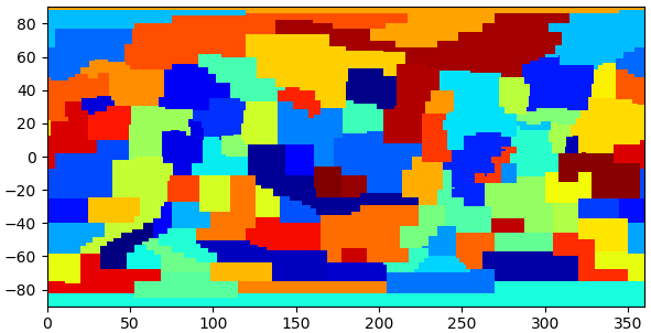
大体こんな感じです。国家の領域と似て、あまりにも不平等な面積ですね。
ただし、赤道座標はどんどん変わっていくものです。星座の定義に使われるのは1875年の時の赤道です。現在一般に使われている赤道は2000年の赤道を元とする国際天文基準座標系(ICRS)です。百年も経ったら座標は僅かずれているので、星座を考える時は座標変換が必要です。
座標の変換
座標変換は随分複雑なことですが、astropyでは座標の処理のために使うastropy.coordinatesというサブモジュールが含まれています。これを使ったら座標変換は簡単です。
例えば1875年の時の天の北極はICRS座標での位置はどこなのか知りたい場合はこうすることができます。
from astropy.coordinates import SkyCoord,PrecessedGeocentric

b1875 = PrecessedGeocentric(equinox='B1875')
b1875_hokkyoku = SkyCoord(ra=0,dec=90,unit='deg',frame=b1875)
b1875_hokkyoku_icrs = b1875_hokkyoku.transform_to('icrs')
print(b1875_hokkyoku_icrs)
<SkyCoord (ICRS): (ra, dec) in deg
    (180.72688238, 89.30964892)>
1875年の北極点は2000年になると90度から89.3度に移動しているようです。0.7度の差は僅かなように見えますが、計算する時に大きな違いを起こせるので、注意しないといけないものです。
get_constellationで星座を取得
特定の位置がどの星座に属するかを知りたければ、まずは座標を変換して上述の表を使ったらいいですが、それを計算する関数はastropyには含まれているので、簡単にできます。
(そもそもその表はこの関数によって使われるためのもので、私達が勝手に直接見るためのものではなかったのですが)
SkyCoordクラスのオブジェクトのget_constellationというメソッドを使えばその位置の属する星座をわかります。
例えば、天の北極と南極の星座を見ます。
hokkyoku = SkyCoord(ra=0,dec=90,unit='deg')
print(hokkyoku.get_constellation())
nankyoku = SkyCoord(ra=0,dec=-90,unit='deg')
print(nankyoku.get_constellation())
Ursa Minor
Octans
天球上の星座区分
次はget_constellationを使って天球上の各領域の星座を表示します。SkyCoordはnumpyのndarrayと共に使うことができるので、赤経と赤緯のmeshgridを作って全域の星座を一気に求めることができます。
import numpy as np

ra,dec = np.meshgrid(np.linspace(0,360,361),np.linspace(-90,90,181))
tenkyuu = SkyCoord(ra=ra,dec=dec,unit='deg')
seiza = tenkyuu.ravel().get_constellation().reshape(*ra.shape) # 星座の名前を求める
z = (seiza[:,:,None]==np.unique(seiza)).argmax(2) # 星座の名前を数字に変換
plt.figure(figsize=[7,4])
plt.gca(aspect=1)
plt.contour(ra,dec,z,88,colors='k',linestyles=':',linewidths=0.1)
plt.pcolormesh(ra,dec,z,cmap='jet')
plt.show()
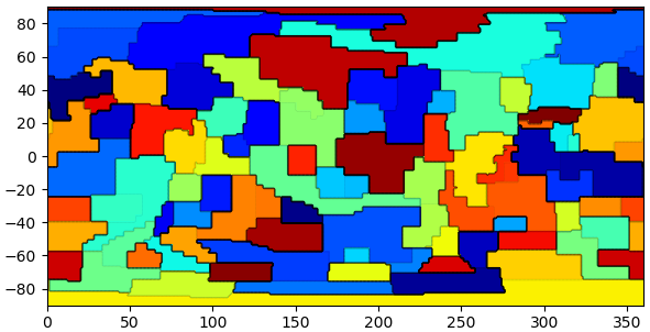
結果はさっきと比べたらあまり変わらないが、僅かずれているようには見えます。
次はxyz座標に変換して三次元でプロットしてみます。
from mpl_toolkits.mplot3d import Axes3D
import imageio

mx,my,mz = tenkyuu.cartesian.xyz # xyz座標に変換
iro = np.stack([z/87,z%5/4,1-z%4/4],2) # できるだけ各星座に違う色をつける
fig = plt.figure(figsize=[6,6])
ax = plt.axes([0,0,1,1],projection='3d',xlim=[-0.6,0.6],ylim=[-0.6,0.6],zlim=[-0.6,0.6],facecolor='k')
ax.plot_surface(mx,my,mz,facecolors=iro,rstride=1,cstride=1,alpha=0.9)
plt.axis('off') # 軸を隠す

gif = [] # どんどん回してアニメーションgifを作る
for i in range(24):
    ax.view_init(30*np.sin(i*np.pi/12),i*15) # 眺める角度を変える
    fig.canvas.draw()
    gif.append(np.array(fig.canvas.renderer._renderer))
plt.close()
imageio.mimsave('seiza_kubun.gif',gif,fps=5) # 保存
こんな感じで天球は区分されているのです。
各星座にある星を表示する
次は各星座に属する星を見てみたいです。星のデータは色んなウェブサイトから取得できます。ここでは天文学者によく使われている星のデータベースを持つsimbadというサイトからのデータを使います。
astropyの付属モジュールであるastroqueryを使ったら手動でサイトから検索してダウンロードする必要がなくsimbadのデータを取得できます。
ここでsimbadから等級5以下の星を取得してみます。
from astroquery.simbad import Simbad

simbad = Simbad()
simbad.add_votable_fields('flux(V)')
hoshi = simbad.query_criteria('Vmag<5',otype='star')
print(hoshi)
  MAIN_ID         RA           DEC      ...     COO_BIBCODE     FLUX_V
               "h:m:s"       "d:m:s"    ...                      mag
----------- ------------- ------------- ... ------------------- ------
  HD   5015 00 53 04.1958 +61 07 26.301 ... 2018yCat.1345....0G    4.8
  * nu. Sco 16 11 59.7356 -19 27 38.536 ... 2007A&A...474..653V    4.0
* pi.02 UMa 08 40 12.8204 +64 19 40.573 ... 2018yCat.1345....0G   4.61
  * tet Cen 14 06 40.9475 -36 22 11.837 ... 2007A&A...474..653V   2.05
  * del Cap 21 47 02.4442 -16 07 38.233 ... 2007A&A...474..653V   2.83
    * n Vel 08 41 13.1296 -47 19 01.661 ... 2018yCat.1345....0G   4.77
        ...           ...           ... ...                 ...    ...
  * mu. Sgr 18 13 45.8088 -21 03 31.794 ... 2007A&A...474..653V   3.85
  * ups Dra 18 54 23.8581 +71 17 49.855 ... 2018yCat.1345....0G  4.814
  * bet Cha 12 18 20.8245 -79 18 44.070 ... 2007A&A...474..653V  4.229
  * h02 Sgr 19 36 42.4328 -24 53 01.028 ... 2007A&A...474..653V  4.598
  * del Ser 15 34 48.1476 +10 32 19.924 ... 2007A&A...474..653V   3.79
  * ups Leo 11 36 56.9308 -00 49 25.496 ... 2007A&A...474..653V    4.3
  * del Her 17 15 01.9105 +24 50 21.145 ... 2007A&A...474..653V   3.13
Length = 1748 rows
simbadのデータは星の他に星団や銀河や星雲も含まれていますが、otype='star'を指定することで星だけに絞ります。
結果に1748の星が出ますが、実は重複している星もあります。連星であるシリウスはこのデータには個別のalf CMa Aと総合のalf CMaがあります。ケンタウルス座α星も同じように重複しています。
print(hoshi[hoshi['FLUX_V']<0.2])
  MAIN_ID         RA           DEC      ...     COO_BIBCODE     FLUX_V
               "h:m:s"       "d:m:s"    ...                      mag
----------- ------------- ------------- ... ------------------- ------
* alf CMa A  06 45 08.917  -16 42 58.02 ... 2002A&A...384..180F  -1.09
  * alf Boo 14 15 39.6720 +19 10 56.673 ... 2007A&A...474..653V  -0.05
  * bet Ori 05 14 32.2721 -08 12 05.898 ... 2007A&A...474..653V   0.13
* alf Cen A 14 39 36.4940 -60 50 02.373 ... 2007A&A...474..653V   0.01
  * alf Cen  14 39 36.204  -60 50 08.23 ...                       -0.1
  * alf Lyr 18 36 56.3363 +38 47 01.280 ... 2007A&A...474..653V   0.03
  * alf CMa 06 45 08.9172 -16 42 58.017 ... 2007A&A...474..653V  -1.46
  * alf Aur 05 16 41.3587 +45 59 52.769 ... 2007A&A...474..653V   0.08
  * alf Car 06 23 57.1098 -52 41 44.381 ... 2007A&A...474..653V  -0.74
ここで重複していても何の損もないので大目に見ます。
赤道座標で各星座の星を違う色で表示してみます。
sc = SkyCoord(ra=hoshi['RA'],dec=hoshi['DEC'],unit=['hourangle','deg'])
seiza = sc.get_constellation()
ra,dec = sc.ra,sc.dec
z = (seiza[:,None]==np.unique(seiza)).argmax(1)
iro = np.stack([z/87,z%5/4,1-z%4/4],1)
s = (5-hoshi['FLUX_V'])*3

plt.figure(figsize=[8,4])
plt.gca(xlim=[0,360],ylim=[-90,90],aspect=1,facecolor='k')
plt.scatter(ra,dec,c=iro,s=s)
plt.show()
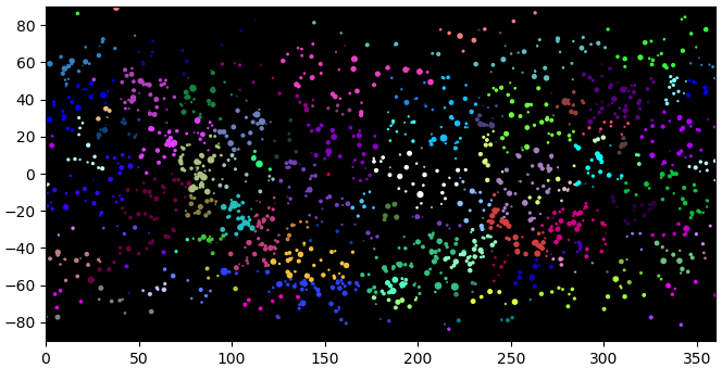
意外と多すぎてわかりにくいようです。
有名な星座を個別に例として見てみます。
まずは一番わかりやすい星座であるオリオン座
plt.gca(facecolor='k',aspect=1,title='Orion')
o = (seiza=='Orion')
plt.scatter(ra[o],dec[o],c='w',s=s[o])
plt.show()
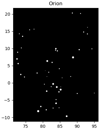
立派な猟師の姿です。
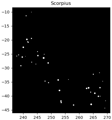
次はわかりやすい「?」の形をするさそり座
plt.gca(facecolor='k',aspect=1,title='Scorpius')
o = (seiza=='Scorpius')
plt.scatter(ra[o],dec[o],c='w',s=s[o])
plt.show()
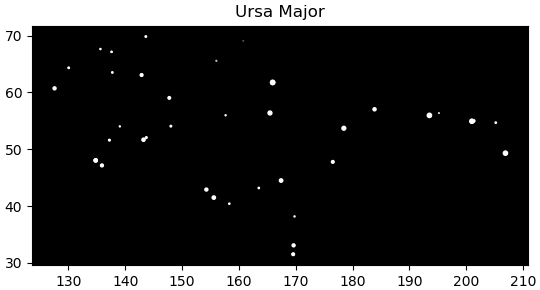
plt.gca(facecolor='k',aspect=1,title='Ursa Major')
o = (seiza=='Ursa Major')
plt.scatter(ra[o],dec[o],c='w',s=s[o])
plt.show()
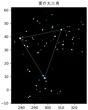
plt.gca(facecolor='k',aspect=1)
o = (seiza=='Lyra')
plt.scatter(ra[o],dec[o],c='#ffffaa',s=s[o])
vega = ra[o][s[o].argmax()].value,dec[o][s[o].argmax()].value
o = (seiza=='Aquila')
plt.scatter(ra[o],dec[o],c='#aaffff',s=s[o])
altair = ra[o][s[o].argmax()].value,dec[o][s[o].argmax()].value
o = (seiza=='Cygnus')
plt.scatter(ra[o],dec[o],c='#aaffaa',s=s[o])
deneb = ra[o][s[o].argmax()].value,dec[o][s[o].argmax()].value
plt.plot([vega[0],altair[0],deneb[0],vega[0]],[vega[1],altair[1],deneb[1],vega[1]],'--w',lw=0.5)
plt.title('夏の大三角',fontname='AppleGothic')
plt.show()
次は三次元で星をプロットします。
x,y,z = sc.cartesian.xyz
fig = plt.figure(figsize=[6,6])
ax = plt.axes([0,0,1,1],projection='3d',xlim=[-0.6,0.6],ylim=[-0.6,0.6],zlim=[-0.6,0.6],facecolor='k')
ax.scatter(x,y,z,c=iro,s=s)
ra,dec = np.meshgrid(np.linspace(0,360,25),np.linspace(-90,90,13))
gx,gy,gz = SkyCoord(ra=ra,dec=dec,unit='deg').cartesian.xyz
ax.plot_wireframe(gx,gy,gz,color='#444444',linestyle='-') # 赤経と赤緯の線
ax.plot([0,0],[0,0],[-1.2,1.2],'#444444') # 中央の軸
plt.axis('off')
gif = []
for i in range(50):
    ax.view_init(30,i*360/50)
    fig.canvas.draw()
    gif.append(np.array(fig.canvas.renderer._renderer))
plt.close()
imageio.mimsave('seiza.gif',gif,fps=4)
星座の面積
見ての通り星座の面積はばらばらです。どの星座がどんなに大きいか知っておきたいです。
実はwikiとか見たらすぐわかります https://ja.wikipedia.org/wiki/星座の広さ順の一覧
ここでは簡単なモンテカルロ法を使って面積を計算してみます。たくさんな位置をランダムしてその位置の星座を求めます。星座に広い面積があればあるほどランダムされた位置はその星座に入りやすく、入った数で面積を推測できます。
勿論、モンテカルロ法でできた結果は正確な答えではなく、ランダムによってある程度の誤差があります。ランダムの数は多いほど答えは実際と近い。
すべての方向が同じ分布をするためには一様分布ではなく正規分布をランダムに使います。
百万くらいランダムして結果を見ます。
x,y,z = np.random.randn(3,1000000)
seiza = SkyCoord(x,y,z,representation_type='cartesian').get_constellation()
percent = sorted(('%.4f%%%20s'%(list(seiza).count(c)/10000,c) for c in set(seiza)),reverse=True)
print('\n'.join(percent))
3.1548%               Hydra
3.1290%               Virgo
3.0908%          Ursa Major
2.9779%               Cetus
2.9626%            Hercules
2.7738%            Eridanus
2.7058%             Pegasus
2.6237%               Draco
2.5845%           Centaurus
2.3952%            Aquarius
2.3063%            Ophiucus
2.2964%                 Leo
2.2044%              Boötes
2.1643%              Pisces
2.1200%         Sagittarius
1.9436%              Cygnus
1.9205%              Taurus
1.8265%      Camelopardalis
1.7484%           Andromeda
1.6097%              Puppis
1.5765%              Aquila
1.5731%              Auriga
1.5548%             Serpens
1.5010%             Perseus
1.4672%          Cassiopeia
1.4530%               Orion
1.4262%             Cepheus
1.3217%                Lynx
1.3166%               Libra
1.2658%              Gemini
1.2352%              Cancer
1.2143%                Vela
1.2111%            Scorpius
1.1859%              Carina
1.1763%           Monoceros
1.1464%            Sculptor
1.1458%             Phoenix
1.1261%      Canes Venatici
1.0619%               Aries
1.0048%         Capricornus
0.9708%              Fornax
0.9297%         Canis Major
0.9261%      Coma Berenices
0.9066%                Pavo
0.8746%                Grus
0.7946%               Lupus
0.7622%             Sextans
0.7159%              Tucana
0.7104%               Lepus
0.7052%              Octans
0.7012%                Lyra
0.6976%               Indus
0.6824%              Crater
0.6521%           Vulpecula
0.6508%             Columba
0.6179%          Ursa Minor
0.6033%          Horologium
0.5975%         Telescopium
0.5954%              Pictor
0.5910%    Pisces Austrinus
0.5807%              Hydrus
0.5801%              Antlia
0.5699%                 Ara
0.5608%           Leo Minor
0.5337%               Pyxis
0.5086%                Apus
0.5064%        Microscopium
0.4905%             Lacerta
0.4555%           Delphinus
0.4551%              Corvus
0.4507%         Canis Minor
0.4347%     Corona Borealis
0.4318%              Dorado
0.4076%               Norma
0.3755%               Mensa
0.3420%              Volans
0.3338%               Musca
0.3145%          Triangulum
0.3082%           Chamaleon
0.3074%              Caelum
0.3064%    Corona Australis
0.2684%           Reticulum
0.2677% Triangulum Australe
0.2632%              Scutum
0.2271%            Circinus
0.1913%             Sagitta
0.1749%            Equuleus
0.1663%               Crux
一番大きいのはうみへび座で、一番小さいのはみなみじゅうじ座で、答えは大体実際と一致しています。
終わりに
以上astropyをいじって色々試した結果です。使いこなせたらもっと色んなことができるようです。