はじめに
本記事シリーズではSERVIRが以下のサイトで公開している「SAR Handbook」を写経し、理解を深めることを目的としています。
https://servirglobal.net/resources/sar-handbook
もともとのサイトや資料は英語にて記載されているので、翻訳しつつコード理解をしていきます。
以下の記事の続きで、本記事ではChapter3のPart5について記載します。
https://qiita.com/oz_oz/items/0238dd7922fe381d7976
CHAPTER3
Using SAR Data for Mapping Deforestation and Forest Degradation
Chp3の説明資料は以下にあります。
https://gis1.servirglobal.net/TrainingMaterials/SAR/Ch3-Content.pdf
Chp3では主にSARによる森林監視について触れており、Sentinel-1などのSARミッションの登場により、適切な前処理と変化検出手法を用いることで、中解像度での森林監視が実現可能となったことを説明しています。
SAR Training Workshop for Forest Applications
Chp3の問題資料は以下にあります。
https://gis1.servirglobal.net/TrainingMaterials/SAR/3B_TrainingModule.pdf
Jupyter Notebook形式の資料は以下にあります。
https://gis1.servirglobal.net/TrainingMaterials/SAR/Scripts_ch3.zip
PART 5 - SAR/Optical (NDVI) Time Series Analysis
Josef Kellndorfer, Ph.D., President and Senior Scientist, Earth Big Data, LLC
Revision date: January 2018
In this chapter we compare time series data of C-band Backscatter and Landsat 8 NDVI over a forested site in Southern Niger.
本章では、ニジェール南部の森林地帯におけるCバンド後方散乱とLandsat-8のNDVIの時系列データを比較します。
# Importing relevant python packages
import pandas as pd
import gdal
import numpy as np
import time,os
from skimage import exposure # to enhance image display

# For plotting
%matplotlib inline
import matplotlib.pylab as plt
import matplotlib.patches as patches
import matplotlib.cm as cm

font = {'family' : 'monospace',
          'weight' : 'bold',
          'size'   : 18}
plt.rc('font',**font)

# Define a helper function for a 4 part figure with backscatter, NDVI and False Color Infrared
def ebd_plot(bandnbrs):
    fig,ax=plt.subplots(2,2,figsize=(16,16))
    # Bands for sentinel and landsat:
    # Sentinel VV
    sentinel_vv=img_handle[0].GetRasterBand(bandnbrs[0]).ReadAsArray(*subset_sentinel)
    sentinel_vv=20.*np.log10(sentinel_vv)-83 # Covert to dB
    # Sentinel VH
    sentinel_vh=img_handle[1].GetRasterBand(bandnbrs[0]).ReadAsArray(*subset_sentinel)
    sentinel_vh=20.*np.log10(sentinel_vh)-83 # Covert to dB
    # # Landsat False Color InfraRed
    r=img_handle[5].GetRasterBand(bandnbrs[1]).ReadAsArray(*subset_landsat)/10000.
    g=img_handle[4].GetRasterBand(bandnbrs[1]).ReadAsArray(*subset_landsat)/10000.
    b=img_handle[3].GetRasterBand(bandnbrs[1]).ReadAsArray(*subset_landsat)/10000.
    fcir=np.dstack((r,g,b))
    for i in range(fcir.shape[2]):
        fcir[:,:,i] = exposure.\
        equalize_hist(fcir[:,:,i],
        mask=~np.equal(fcir[:,:,i],-.9999))
    # Landsat NDVI
    landsat_ndvi=img_handle[2].GetRasterBand(bandnbrs[1]).ReadAsArray(*subset_landsat)
    mask=landsat_ndvi==-9999
    landsat_ndvi = landsat_ndvi/10000. # Scale to real NDVI value
    landsat_ndvi[mask]=np.nan
    svv = ax[0][0].imshow(sentinel_vv,cmap='jet',vmin=np.nanpercentile(sentinel_vv,5),
                   vmax=np.nanpercentile(sentinel_vv,95))
    cb = fig.colorbar(svv,ax=ax[0][0],orientation='horizontal')
    cb.ax.set_title('C-VV $\gamma^o$ [dB]')
    svh = ax[0][1].imshow(sentinel_vh,cmap='jet',vmin=np.nanpercentile(sentinel_vh,5),
                   vmax=np.nanpercentile(sentinel_vh,95))
    cb = fig.colorbar(svh,ax=ax[0][1],orientation='horizontal')
    cb.ax.set_title('C-VH $\gamma^o$ [dB]')

    nvmin=np.nanpercentile(landsat_ndvi,5)
    nvmax=np.nanpercentile(landsat_ndvi,95)
    # nvmin=-1
    # nvmax=1
    nax = ax[1][0].imshow(landsat_ndvi,cmap='jet',vmin=nvmin,
                   vmax=nvmax)
    cb = fig.colorbar(nax,ax=ax[1][0],orientation='horizontal')
    cb.ax.set_title('NDVI')

    fc= ax[1][1].imshow(fcir)
    # cb = fig.colorbar(fc,cmap=cm.gray,ax=ax[1][1],orientation='horizontal')
    # cb.ax.set_title('False Color Infrared')

    ax[0][0].axis('off')
    ax[0][1].axis('off')
    ax[1][0].axis('off')
    ax[1][1].axis('off')
    ax[0][0].set_title('Sentinel-1 C-VV {}'.format(stindex[bandnbrs[0]-1].date()))
    ax[0][1].set_title('Sentinel-1 C-VH {}'.format(stindex[bandnbrs[0]-1].date()))
    ax[1][0].set_title('Landsat-8 NDVI {}'.format(ltindex[bandnbrs[1]-1].date()))
    ax[1][1].set_title('Landsat-8 False Color IR {}'.format(ltindex[bandnbrs[1]-1].date()))
    _=fig.suptitle('Sentinel-1 Backscatter and Landsat NDVI and FC IR',size=16)
このコードではSentinel-1およびLandsat-8の衛星データを可視化するための関数「ebd_plot」を定義しています。この関数は、特定のバンド番号に対して4つの画像(Sentinel-1のVVおよびVHの後方散乱、Landsat-8のNDVIおよびFalse Color Infrared)を表示します。
関数の中身を見ていきます。
fig, ax = plt.subplots(2, 2, figsize=(16, 16))
2*2の合計4つのサブプロットを持つ図を作成します。
# Bands for sentinel and landsat:
    # Sentinel VV
    sentinel_vv=img_handle[0].GetRasterBand(bandnbrs[0]).ReadAsArray(*subset_sentinel)
    sentinel_vv=20.*np.log10(sentinel_vv)-83 # Covert to dB
    # Sentinel VH
    sentinel_vh=img_handle[1].GetRasterBand(bandnbrs[0]).ReadAsArray(*subset_sentinel)
    sentinel_vh=20.*np.log10(sentinel_vh)-83 # Covert to dB
sentinel_vvとsentinel_vhは、それぞれVVおよびVH偏波のデータを読み込み、dBスケールに変換しています。
# # Landsat False Color InfraRed
    r=img_handle[5].GetRasterBand(bandnbrs[1]).ReadAsArray(*subset_landsat)/10000.
    g=img_handle[4].GetRasterBand(bandnbrs[1]).ReadAsArray(*subset_landsat)/10000.
    b=img_handle[3].GetRasterBand(bandnbrs[1]).ReadAsArray(*subset_landsat)/10000.
    fcir=np.dstack((r,g,b))
LandsatのFalseColorInfraRedデータ(FCIR)を読み込み、正規化してからヒストグラム均等化を行います。
読み込み時に実査の反射率のスケールにするため10000で割っています。
FalseColorInfraRedデータとは近赤外線、赤、緑のバンドを使用して作成されたデータを指します。
今回の場合、近赤外線:バンド5、赤:バンド4、緑:バンド3をそれぞれr,g,bとして割り当てて表示しています。
    for i in range(fcir.shape[2]):
        fcir[:,:,i] = exposure.\
        equalize_hist(fcir[:,:,i],
        mask=~np.equal(fcir[:,:,i],-.9999))
ヒストグラム均等化を行います。これにより、画像のコントラストが強調され、詳細が見やすくなります。
-9999(無効値)をマスクして均等化の対象外とします。
    # Landsat NDVI
    landsat_ndvi=img_handle[2].GetRasterBand(bandnbrs[1]).ReadAsArray(*subset_landsat)
    mask=landsat_ndvi==-9999
    landsat_ndvi = landsat_ndvi/10000. # Scale to real NDVI value
    landsat_ndvi[mask]=np.nan
LandsatのNDVIデータを読み込み、実際のスケールに戻したうえで無効なデータをマスクしてから正規化します。
    svv = ax[0][0].imshow(sentinel_vv, cmap='jet', vmin=np.nanpercentile(sentinel_vv, 5),
                          vmax=np.nanpercentile(sentinel_vv, 95))
    cb = fig.colorbar(svv, ax=ax[0][0], orientation='horizontal')
    cb.ax.set_title('C-VV $\gamma^o$ [dB]')
    svh = ax[0][1].imshow(sentinel_vh, cmap='jet', vmin=np.nanpercentile(sentinel_vh, 5),
                          vmax=np.nanpercentile(sentinel_vh, 95))
    cb = fig.colorbar(svh, ax=ax[0][1], orientation='horizontal')
    cb.ax.set_title('C-VH $\gamma^o$ [dB]')

    nvmin = np.nanpercentile(landsat_ndvi, 5)
    nvmax = np.nanpercentile(landsat_ndvi, 95)
    nax = ax[1][0].imshow(landsat_ndvi, cmap='jet', vmin=nvmin,
                          vmax=nvmax)
    cb = fig.colorbar(nax, ax=ax[1][0], orientation='horizontal')
    cb.ax.set_title('NDVI')

    fc = ax[1][1].imshow(fcir)

    ax[0][0].axis('off')
    ax[0][1].axis('off')
    ax[1][0].axis('off')
    ax[1][1].axis('off')
    ax[0][0].set_title('Sentinel-1 C-VV {}'.format(stindex[bandnbrs[0] - 1].date()))
    ax[0][1].set_title('Sentinel-1 C-VH {}'.format(stindex[bandnbrs[0] - 1].date()))
    ax[1][0].set_title('Landsat-8 NDVI {}'.format(ltindex[bandnbrs[1] - 1].date()))
    ax[1][1].set_title('Landsat-8 False Color IR {}'.format(ltindex[bandnbrs[1] - 1].date()))
    _ = fig.suptitle('Sentinel-1 Backscatter and Landsat NDVI and FC IR', size=16)
各サブプロットに画像を表示し、カラーバーを追加しています。
また、各サブプロットのタイトルと軸の設定を行います。
Set Project Directory and Filenames
West Africa - Biomass Site
datadirectory='/Users/josefk/servir_data/wa/BIOsS1'
datadirectory='/dev/shm/projects/c401servir/wa/BIOsS1'
sentinel1_datefile='S32631X398020Y1315440sS1_A_vv_0001_mtfil.dates'
sentinel1_imagefile='S32631X398020Y1315440sS1_A_vv_0001_mtfil.vrt'
sentinel1_imagefile_cross='S32631X398020Y1315440sS1_A_vh_0001_mtfil.vrt'
landsat8_ndvi='landsat/L8_192_052_NDVI.vrt'
landsat8_b3='landsat/L8_192_052_B3.vrt'
landsat8_b4='landsat/L8_192_052_B4.vrt'
landsat8_b5='landsat/L8_192_052_B5.vrt'
landsat8_datefile='landsat/L8_192_052_NDVI.dates'
Acquisition Dates
Read from the Dates file the dates in the time series and make a pandas date index
Dates ファイルから時系列の日付を読み取り、パンダの日付インデックスを作成します。
sdates=open(sentinel1_datefile).readlines()
stindex=pd.DatetimeIndex(sdates)
j=1
print('Bands and dates for',sentinel1_imagefile)
for i in stindex:
    print("{:4d} {}".format(j, i.date()),end=' ')
    j+=1
    if j%5==1: print()

ldates=open(landsat8_datefile).readlines()
ltindex=pd.DatetimeIndex(ldates)
j=1
print('Bands and dates for',landsat8_ndvi)
for i in ltindex:
    print("{:4d} {}".format(j, i.date()),end=' ')
    j+=1
    if j%5==1: print()

上記のコードは前回以前のChapterでも同じことをしているので詳しい説明は割愛します。
Projection and Georeferencing Information of the SAR and Optical Time Series Data Stacks
For processing of the imagery in this notebook we generate a list of image handles and retrieve projection and georeferencing information. We print out the retrieved information.
このノートブックの画像を処理するために、画像ハンドルのリストを生成し、投影情報と地理参照情報を取得します。取得した情報を印刷します。
画像ハンドルとは、画像ファイルへの参照を持つオブジェクトで、これを使って画像データにアクセスします。
画像ハンドルのリストを生成することで、複数の画像ファイルを効率的に管理し処理することができます。
投影法情報は地球表面をどのように平面に投影するかを示す情報です。
地理参照情報は画像内の各ピクセルが地球上のどの位置に対応するかを示す情報です。
これらの情報を取得することで、画像データを地理的に正確な位置に配置し、解析や表示を行うことができます。
imagelist=[sentinel1_imagefile,sentinel1_imagefile_cross,landsat8_ndvi,landsat8_b3,landsat8_b4,landsat8_b5]
geotrans=[]
proj=[]
img_handle=[]
xsize=[]
ysize=[]
bands=[]
for i in imagelist:
    img_handle.append(gdal.Open(i))
    geotrans.append(img_handle[-1].GetGeoTransform())
    proj.append(img_handle[-1].GetProjection())
    xsize.append(img_handle[-1].RasterXSize)
    ysize.append(img_handle[-1].RasterYSize)
    bands.append(img_handle[-1].RasterCount)
# for i in proj:
#     print(i)
# for i in geotrans:
#     print(i)
# for i in zip(['C-VV','C-VH','NDVI','B3','B4','B5'],bands,ysize,xsize):
#     print(i)
imagelistは、処理対象の画像ファイルのリストです。
このリストには、Sentinel-1のVVとVHの2つのバンド、Landsat-8のNDVI、B3、B4、B5の4つのバンドが含まれています。
各行の意味は以下になります。
- for i in imagelist: imagelist内の各画像ファイルに対してループを実行
- img_handle.append(gdal.Open(i)): 画像ファイルを開いてハンドルを取得し、img_handleリストに追加
- geotrans.append(img_handle[-1].GetGeoTransform()): 最新の画像ハンドルからジオトランスフォーム情報を取得し、geotransリストに追加
- proj.append(img_handle[-1].GetProjection()): 最新の画像ハンドルから投影法情報を取得し、projリストに追加
- xsize.append(img_handle[-1].RasterXSize): 最新の画像ハンドルから画像のX方向のサイズを取得し、xsizeリストに追加
- ysize.append(img_handle[-1].RasterYSize): 最新の画像ハンドルから画像のY方向のサイズを取得し、ysizeリストに追加
- bands.append(img_handle[-1].RasterCount): 最新の画像ハンドルから画像のバンド数を取得し、bandsリストに追加
情報出力の部分はコメントアウトされていますが、処理の中身は以下になります。
- projリスト内の各投影法情報を出力
- geotransリスト内の各ジオトランスフォーム情報を出力
- zip関数を使って、バンド名、バンド数、画像のY方向サイズ、X方向サイズをペアにして出力
Display SAR and NDVI Images
First, depending on the capacity of the computer we might want to define a subset. We will choose the subset in the raster extension of the Sentinel-1 Image and use the geotransformation information to extract the corresponding subset in the Landsat Image. We assume that the images have the same upper left coordinate. The we can compute the offsets and extent in the Landsat image as follows:
We can use these calibration factors to get the landsat subset as follows


最初に、コンピュータの能力に応じて、サブセットを定義したい場合があります。Sentinel-1画像のラスター拡張で部分集合を選び、地形変換情報を使ってLandsat画像の対応する部分集合を抽出します。画像は同じ左上座標を持つと仮定するとLandsat画像のオフセットとエクステントは以下のように計算できます。
x_{\text{cal}} = \frac{x_{\text{res}_{\text{sentinel-1}}}}{x_{\text{res}_{\text{landsat}}}}
y_{\text{cal}} = \frac{y_{\text{res}_{\text{sentinel-1}}}}{y_{\text{res}_{\text{landsat}}}}
これらの校正係数を用いて、Landsatサブセットを次のように求めることができます。
x_{\text{off}_{\text{landsat}}} = x_{\text{off}_{\text{sentinel-1}}} \times x_{\text{cal}}
y_{\text{off}_{\text{landsat}}} = y_{\text{off}_{\text{sentinel-1}}} \times y_{\text{cal}}
x_{\text{size}_{\text{landsat}}} = x_{\text{size}_{\text{sentinel-1}}} \times x_{\text{cal}}
y_{\text{size}_{\text{landsat}}} = y_{\text{size}_{\text{sentinel-1}}} \times y_{\text{cal}}
意訳すると上記のとおりですが、難しい単語が多いのでもう少し詳細に記載します。
- サブセットを定義する理由
画像全体を処理するのはデータ量が多く、コンピュータの処理能力を超える可能性があります。そのため、特定の部分(サブセット)だけを処理することで、効率的にデータを扱います。 - Sentinel-1画像のサブセットを選択
最初に、Sentinel-1画像の中で処理したい領域を選択します。これは、ラスターデータ(格子状のデータ)の一部を選び出すことを意味します。 - ジオトランスフォーメーション情報の利用
ジオトランスフォーメーション情報とは、画像の各ピクセルが地球上のどの位置に対応するかを示す情報です。これを使って、Landsat画像の中で対応する部分を特定します。 - Landsat画像のサブセットを抽出
Sentinel-1画像のサブセットに対応するLandsat画像の部分を抽出するために、Landsat画像のオフセットとサイズを計算します。 - 上左座標の仮定
ここでは、Sentinel-1画像とLandsat画像が同じ左上座標(上端と左端の交点)を持っていると仮定します。これにより、対応するサブセットの位置を簡単に計算できます。 - オフセット(始点)の計算
Sentinel-1画像のサブセットの開始点を基に、Landsat画像の開始点(オフセット)を計算します。
x_{\text{off}_{\text{landsat}}} = x_{\text{off}_{\text{sentinel-1}}} \times x_{\text{cal}}
y_{\text{off}_{\text{landsat}}} = y_{\text{off}_{\text{sentinel-1}}} \times y_{\text{cal}}
- サイズ(範囲)の計算
Sentinel-1画像のサブセットのサイズを基に、Landsat画像のサイズ(範囲)を計算します。
x_{\text{size}_{\text{landsat}}} = x_{\text{size}_{\text{sentinel-1}}} \times x_{\text{cal}}
y_{\text{size}_{\text{landsat}}} = y_{\text{size}_{\text{sentinel-1}}} \times y_{\text{cal}}
この方法により、Sentinel-1画像の一部(サブセット)を基にして、対応するLandsat画像のサブセットを正確に抽出することができます。
両方の画像の特定の領域を比較・解析することが可能であり、異なる解像度やスケールの衛星画像を統合して解析する際に有用です。
subset_sentinel=None
subset_sentinel=(570,40,500,500)  # Adjust or comment out if you don't want a subset
if subset_sentinel == None:
    subset_sentinel=(0,0,img_handle[0].RasterXSize,img_handle[0].RasterYSize)
    subset_landsat=(0,0,img_handle[2].RasterXSize,img_handle[2].RasterYSize)
else:
    xoff,yoff,xsize,ysize=subset_sentinel
    xcal=geotrans[0][1]/geotrans[2][1]
    ycal=geotrans[0][5]/geotrans[2][5]
    subset_landsat=(int(xoff*xcal),int(yoff*ycal),int(xsize*xcal),int(ysize*ycal))

print('Subset Sentinel-1',subset_sentinel,'\nSubset Landsat   ',subset_landsat)
Subset Sentinel-1 (570, 40, 500, 500)
Subset Landsat (380, 26, 333, 333)
上記のコードは解説どおりですがステップを示すと以下になります。
- subset_sentinelに特定の値(570,40,500,500)を設定
これは、Sentinel-1画像のサブセットのオフセット(始点)とサイズ(範囲)を指定しています。 - サブセットが設定されている場合とされていない場合で処理分岐
- 設定されていない場合
subset_sentinelもsubset_landsat共に画像全体が対象となります。
始点は(0,0)とし、サイズは画像全体のXサイズとYサイズを使用しています。 - 設定されている場合
- キャリブレーションを計算
- xcal = geotrans[0][1] / geotrans[2][1]: X方向のキャリブレーション係数
- ycal = geotrans[0][5] / geotrans[2][5]: Y方向のキャリブレーション係数
- Sentinel-1のサブセットに対応するLandsat画像のサブセットを計算
- int(xoff * xcal): Xオフセットにキャリブレーション係数を掛けて、整数値に変換
- int(yoff * ycal): Yオフセットにキャリブレーション係数を掛けて、整数値に変換
- int(xsize * xcal): Xサイズにキャリブレーション係数を掛けて、整数値に変換
- int(ysize * ycal): Yサイズにキャリブレーション係数を掛けて、整数値に変換
- キャリブレーションを計算
- 設定されていない場合
- 設定されたSentinel-1のサブセット領域とそれに対応するLandsatのサブセット領域を表示
geotransに格納されている値をどのように使ってキャリブレーションしているのかを更に詳細化しようと思います。
geotrans の中身は、ジオトランスフォーム(地理変換)情報を表す6つのパラメータから成ります。これらのパラメータは、ラスターデータ(画像)の地理的な位置と解像度を定義します。
具体的には、次のようなパラメータを持っています。
- x_min: 左上コーナーのX座標(地理座標系)
- pixel_width: ピクセルの幅(地理座標系)
- rotation_x: 回転(通常は0)
- y_min: 左上コーナーのY座標(地理座標系)
- rotation_y: 回転(通常は0)
- pixel_height: ピクセルの高さ(地理座標系、通常負の値)
これを元にして、ピクセル座標から地理座標を計算するための線形変換を行っています。
キャリブレーション係数の計算とサブセットの計算例
仮に geotrans が次のような値を持っていたとします。
- Sentinel-1
geotrans_sentinel = [1000000.0, 10.0, 0.0, 2000000.0, 0.0, -10.0] - Landsat
geotrans_landsat = [1000000.0, 30.0, 0.0, 2000000.0, 0.0, -30.0]
キャリブレーション係数はSentinel-1とLandsatのピクセルサイズの比率を計算することで得られます。
- x方向のキャリブレーション係数(xcal)
xcal = geotrans_sentinel[1] / geotrans_landsat[1] - y方向のキャリブレーション係数 (ycal)
ycal = geotrans_sentinel[5] / geotrans_landsat[5]
geotrans_sentinel[1] -> Sentinel-1 画像のピクセルの幅
geotrans_landsat[1] -> Landsat 画像のピクセルの幅
geotrans_sentinel[5] -> Sentinel-1 画像のピクセルの高さ
geotrans_landsat[5] -> Landsat 画像のピクセルの高さ
この場合キャリブレーション係数は以下となります。
xcal = 10.0 / 30.0 = 0.3333
ycal = -10.0 / -30.0 = 0.3333
サブセットの計算は指定した値に上記のキャリブレーション係数をかけるだけです。
subset_sentinel = (570, 40, 500, 500)
xoff, yoff, xsize, ysize = subset_sentinel
とすると、subset_landsatは以下の計算になります。
subset_landsat = (
int(xoff * xcal), # 570 * 0.3333 ≈ 190
int(yoff * ycal), # 40 * 0.3333 ≈ 13
int(xsize * xcal), # 500 * 0.3333 ≈ 167
int(ysize * ycal) # 500 * 0.3333 ≈ 167
)
↓出力結果
Subset Sentinel-1 (570, 40, 500, 500)
Subset Landsat (190, 13, 167, 167) ※geotrans情報が仮値なので実際の結果と値は異なります。
Now we can pick the bands and plot the Sentinel-1 and Landsat NDVI images of the subset. Change the band numbers to the bands we are interested in.
これで、バンドを選択し、サブセットのSentinel-1およびLandsat NDVI画像をプロットできるようになりました。バンド番号を特定のバンドに変更します。
Dry Season Plot
# DRY SEASON PLOT
bandnbrs=(24,24)
ebd_plot(bandnbrs)

Wet Season Plot
# Wet SEASON PLOT
bandnbrs=(40,37)
ebd_plot(bandnbrs)

In the figure above, for band 24 of Sentinel-1 and 24 of NDVI, which was acquired three days after the Sentinel-1 image, there is an inverse relationship. Where Sentinel-1
exhibits low backscatter, NDVI shows relatively higher NDVI. What are the reasons for this in this environment?
上記の図で、Sentinel-1のバンド24とNDVIのバンド24が比較されています。NDVIのデータはSentinel-1の画像が取得された3日後に取得されたものです。これらの画像では逆の関係が見られます。具体的には、Sentinel-1でバックスキャッターが低い領域では、NDVIが高い値を示しています。このような現象がこの環境で見られる理由は何でしょうか?
と聞かれていますが、正直全体的に見ると合致しています。
一部以下の箇所等は確かに逆になっているように見えます。

Cバンドの帯域はVV偏波の後方散乱値は岩石などの地表面に凹凸が大きい箇所や、比較的裸地などで高くなる傾向があります。
NDVI(正規化植生指数)は、植物の健康状態や密度を示す指標です。NDVIは植生が豊かな場所で高くなるため、広葉樹が上記箇所で多く茂っていた可能性があります。ただ、周りの地域はだいたい一致しています。この地域だけ周りと植生の種類が違うと言うには情報が不足しており判断ができませんでした。
Time Series Profiles of C-Band Backscatter and NDVI
We compute the image means of each time step in the time series stack and plot them together.
時系列スタック内の各時間ステップの画像平均を計算し、それらを一緒にプロットします。
Prepare Sentinel-1 and NDVI Data stacks
Sentinel time series stack
caldB=-83
calPwr = np.power(10.,caldB/10.)

s_ts=[]
for idx in (0,1):
    means=[]
    for i in range(bands[idx]):
        rs=img_handle[idx].GetRasterBand(i+1).ReadAsArray(*subset_sentinel)
        # 1. Conversion to Power
        rs_pwr=np.power(rs,2.)*calPwr
        rs_means_pwr = np.mean(rs_pwr)
        rs_means_dB = 10.*np.log10(rs_means_pwr)
        means.append(rs_means_dB)
    s_ts.append(pd.Series(means,index=stindex))
idxが0の場合はVV、1の場合はVHを計算しています。
Sentinel-1のVVおよびVH偏波の各バンドに対して、後方散乱強度をパワーに変換し、その平均値をdBに変換して、時系列データとして保存します。
s_tsリストには、VVおよびVH偏波の時系列データが格納されます。
Landsat NDVI time series stack
means=[]
idx=2
for i in range(bands[idx]):
    r=img_handle[idx].GetRasterBand(i+1).ReadAsArray(*subset_landsat)
    means.append(r[r!=-9999].mean()/10000.)
l_ts=pd.Series(means,index=ltindex)
Landsat画像の各バンドに対して、無効なデータを除外した後、有効なピクセルの平均値を計算し、その値を時系列データとして保存します。
l_tsリストには、Landsatの平均値の時系列データが格納されます。
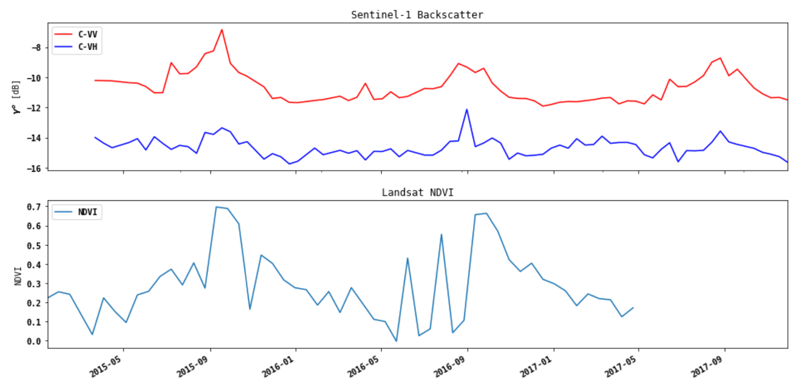
Joint Plot of SAR Backscatter and NDVI of Image Subset Means
Now we plot the time series of the SAR backscatter and NDVI values scaled to the same time axis. We also show the time stamps for the images we display above.
次に、同じ時間軸にスケールされたSAR後方散乱値とNDVI値の時系列をプロットします。上に表示した画像のタイムスタンプも示します。
fig, ax = plt.subplots(2,1,figsize=(16,8))
# ax1.plot(s_ts.index,s_ts.values, 'r-')
s_ts[0].plot(ax=ax[0],color='red',label='C-VV',xlim=(min(min(ltindex),min(stindex)),
                                                     max(max(ltindex),max(stindex))))
s_ts[1].plot(ax=ax[0],color='blue',label='C-VH')
ax[0].set_xlabel('Date')
ax[0].set_ylabel('Sentinel-1 $\gamma^o$ [dB]')

# Make the y-axis label, ticks and tick labels match the line color. ax1.set_ylabel('exp', color='b')
# ax1.tick_params('y', colors='b')
# ax[1] = ax1.twinx()
# s_ts.plot(ax=ax[1],share=ax[0])
l_ts.plot(ax=ax[1],sharex=ax[0],label='NDVI',xlim=(min(min(ltindex),min(stindex)),
                                                     max(max(ltindex),max(stindex))),ylim=(0,0.75))
# ax[1].plot(l_ts.index,l_ts.values,color='green',label='NDVI')
ax[1].set_ylabel('NDVI')
ax[0].set_title('Sentinel-1 Backscatter')
ax[1].set_title('Landsat NDVI')

ax[0].axvline(stindex[bandnbrs[0]-1],color='cyan',label='Sent. Date')
ax[1].axvline(ltindex[bandnbrs[1]-1],color='green',label='NDVI Date')
_=fig.legend(loc='center right')
_=fig.suptitle('Time Series Profiles of Sentinel-1 SAR Backscatter and Landsat-8 NDVI ')
# fig.tight_layout()

上記のコードではおもに以下を処理しています。
- Sentinel-1のプロット
- s_ts[0].plot(...): Sentinel-1のVV偏波の時系列データをプロットし、赤色で表示
- s_ts[1].plot(...): Sentinel-1のVH偏波の時系列データをプロットし、青色で表示
- ax[0].set_xlabel('Date'): x軸のラベルを設定
- ax[0].set_ylabel('Sentinel-1 $\gamma^o$ [dB]'): y軸のラベルを設定
- Landsat-8のプロット
- l_ts.plot(...): Landsat-8のNDVIの時系列データをプロット
sharex=ax[0] は、x軸を上のプロットと共有する設定です。xlim と ylim はそれぞれx軸とy軸の範囲を設定します。 - ax[1].set_ylabel('NDVI'): 下のプロットのy軸のラベルを設定
- l_ts.plot(...): Landsat-8のNDVIの時系列データをプロット
- axvlineを使って、指定した日付に縦線を追加
- stindex[bandnbrs[0] - 1] と ltindex[bandnbrs[1] - 1] はそれぞれSentinel-1とLandsat-8の特定のバンドの日付を指定
仮にbandnbrsが[24, 24]である場合は
stindex[23] -> Sentinel-1の24番目のバンドの日付(23番目のインデックスに対応)
ltindex[23] -> Landsat-8の24番目のバンドの日付(23番目のインデックスに対応)
となります。
Comparison of time series profiles at point locations.
We will pick a pixel location in the SAR image, find the corresponding location in the Landsat NDVI stack and plot the joint time series.
First let's pick a pixel location in the SAR image (i.e. the reference image)
We use the geotrans info to find the same location in the Landsat image
SAR画像内のピクセル位置を選択し、LandsatNDVIスタック内の対応する位置を見つけて、ジョイントタイムシリーズをプロットします。まず、SAR画像(つまり参照画像)内のピクセル位置を選択します。ジオトランス情報を使用して、Landsat画像内の同じ位置を見つけます。
つまり、SAR画像内の特定のピクセル位置を選択し、Landsat NDVIスタック内で対応する位置を見つけ、その位置の時系列データをプロットする方法を示そうとしています。
sarloc=(2000,2000)
ref_x=geotrans[0][0]+sarloc[0]*geotrans[0][1]
ref_y=geotrans[0][3]+sarloc[1]*geotrans[0][5]
print('UTM Coordinates      ',ref_x,ref_y)
print('SAR pixel/line       ',sarloc[0],sarloc[1])
target_pixel=round((ref_x-geotrans[2][0])/geotrans[2][1])
target_line=round((ref_y-geotrans[2][3])/geotrans[2][5])
print('Landsat pixel/line   ',target_pixel,target_line)

上記コードが実施していることを簡単にリストすると以下となります。
- sarloc は、SAR画像内の選択されたピクセル位置を表し、(2000, 2000)の位置を選択
- ref_x は、SAR画像のピクセル位置 (sarloc[0]) を地理座標のX座標に変換した値
- geotrans[0][0] は、SAR画像の左上コーナーのX座標
- geotrans[0][1] は、SAR画像のピクセルの幅
- ref_y は、SAR画像のピクセル位置 (sarloc[1]) を地理座標のY座標に変換した値
- geotrans[0][3] は、SAR画像の左上コーナーのY座標
- geotrans[0][5] は、SAR画像のピクセルの高さ
これにより、SAR画像内のピクセル位置(2000, 2000)が地理座標(ref_x, ref_y)に変換されます。
Landsat側の対応するピクセル位置の計算は説明通りのため割愛しますが、つまるところ、このコードはSAR画像内の特定のピクセル位置(2000, 2000)を選択し、その位置を地理座標(UTM座標)に変換した後、その地理座標を使用して対応するLandsat画像内のピクセル位置を計算しています。このようにして、SAR画像とLandsat画像の同じ地理的位置に対応するピクセルを見つけることができます。
Read the image data at these locations
s_ts_pixel=[]
for idx in (0,1):
    means=[]
    for i in range(bands[idx]):
        rs=img_handle[idx].GetRasterBand(i+1).ReadAsArray(*sarloc,6,6)
        # 1. Conversion to Power
        rs_pwr=np.power(rs,2.)*calPwr
        rs_means_pwr = np.mean(rs_pwr)
        rs_means_dB = 10.*np.log10(rs_means_pwr)
        means.append(rs_means_dB)
    s_ts_pixel.append(pd.Series(means,index=stindex))

means=[]
idx=2
for i in range(bands[idx]):
    r=img_handle[idx].GetRasterBand(i+1).ReadAsArray(target_pixel,target_line,4,4)
    means.append(np.nanmean(r)/10000.)
l_ts_pixel=pd.Series(means,index=ltindex)
Plot the joint time series.
fig, ax = plt.subplots(2,1,figsize=(16,8))
# ax1.plot(s_ts.index,s_ts.values, 'r-')
s_ts[0].plot(ax=ax[0],color='red',label='C-VV',xlim=(min(min(ltindex),min(stindex)),
                                                     max(max(ltindex),max(stindex))))
s_ts_pixel[1].plot(ax=ax[0],color='blue',label='C-VH')
ax[0].set_xlabel('Date')
ax[0].set_ylabel('$\gamma^o$ [dB]')

# Make the y-axis label, ticks and tick labels match the line color. ax1.set_ylabel('exp', color='b')
# ax1.tick_params('y', colors='b')
# ax[1] = ax1.twinx()
# s_ts.plot(ax=ax[1],share=ax[0])
l_ts_pixel.plot(ax=ax[1],sharex=ax[0],label='NDVI',xlim=(min(min(ltindex),min(stindex)),
                                                     max(max(ltindex),max(stindex))))
# ax[1].plot(l_ts.index,l_ts.values,color='green',label='NDVI')
ax[1].set_ylabel('NDVI')
ax[0].set_title('Sentinel-1 Backscatter')
ax[1].set_title('Landsat NDVI')
_=ax[0].legend(loc='upper left')
_=ax[1].legend(loc='upper left')
# fig.tight_layout()
上記のコードはバンドの日付線を引いていないだけで、今まで実施したコードと同様です。
Interprate these time series profiles. While generally the seasonal trends are visible in both like (VV) and cross-polarized (VH) data, and correlate well with the NDVI temporal profile, the cross-polarized response is less pronounced at the example pixel location UTM Coordinates Zone 31N 438020.0 1350960.0.
これらの時系列プロファイルを解釈します。一般に、季節傾向はVVと交差偏波VHデータの両方に見られ、NDVI時間プロファイルとよく相関していますが、交差偏波応答はサンプルのピクセル位置であるUTM座標ゾーン31N 438020.0 1350960.0ではそれほど顕著ではありません。
まとめ
本記事では「SAR Handbook」の3章のトレーニングPart5について写経し、自分なりに理解してみました。
どちらかというと自分のための備忘録として記載しましたが、SARについて勉強し始めたところですので、もし間違っている点等ありましたらコメントいただけると幸いです。