SAR Handbook[Chp3-6]を写経し、難しい単語を使わず意訳してみた

はじめに

本記事シリーズではSERVIRが以下のサイトで公開している「SAR Handbook」を写経し、理解を深めることを目的としています。
https://servirglobal.net/resources/sar-handbook
もともとのサイトや資料は英語にて記載されているので、翻訳しつつコード理解をしていきます。

以下の記事の続きで、本記事ではChapter3のPart5について記載します。
https://qiita.com/oz_oz/items/0238dd7922fe381d7976

CHAPTER3

Using SAR Data for Mapping Deforestation and Forest Degradation

Chp3の説明資料は以下にあります。
https://gis1.servirglobal.net/TrainingMaterials/SAR/Ch3-Content.pdf
Chp3では主にSARによる森林監視について触れており、Sentinel-1などのSARミッションの登場により、適切な前処理と変化検出手法を用いることで、中解像度での森林監視が実現可能となったことを説明しています。

SAR Training Workshop for Forest Applications

Chp3の問題資料は以下にあります。
https://gis1.servirglobal.net/TrainingMaterials/SAR/3B_TrainingModule.pdf
Jupyter Notebook形式の資料は以下にあります。
https://gis1.servirglobal.net/TrainingMaterials/SAR/Scripts_ch3.zip

How to Make RGB Composites from Dual-Polarimetric Data

Josef Kellndorfer, Ph.D., President and Senior Scientist, Earth Big Data, LLC
Revision date: January 2019
In this chapter we introduce how to make a three band color composite and save it

この章では、3バンドのカラー合成を作成し、それを保存する方法を紹介します。

Import Python modules

ライブラリのimportとデータファイルの読み込みを行います。

import os,sys,gdal
%matplotlib inline
import matplotlib.pylab as plt
import matplotlib.patches as patches # Needed to draw rectangles
from skimage import exposure # to enhance image display
import numpy as np
import pandas as pd

# Select the project data set and time series data

# West Africa - Biomass Site
datapath='Users/rmuench/Downloads/wa/BIOsS1/'
datefile='S32631X398020Y1315440sS1_A_vv_0001_mtfil.dates'
imagefile_like='S32631X398020Y1315440sS1_A_vv_0001_mtfil.vrt'
imagefile_cross='S32631X398020Y1315440sS1_A_vh_0001_mtfil.vrt'

os.chdir(datapath)

We are defining two helper functions for this task

• CreateGeoTiff() to write out images
• dualpol2rgb() to compute various metrics from a time series data stack

2つの関数を定義します。

• CreateGeoTiff()：画像を書き出す関数
• dualpol2rgb()：時系列データスタックから様々なメトリクスを計算する関数

def CreateGeoTiff(Name, Array, DataType, NDV,bandnames=None,ref_image=None, 
                  GeoT=None, Projection=None):
    # If it's a 2D image we fake a third dimension:
    if len(Array.shape)==2:
        Array=np.array([Array])
    if ref_image==None and (GeoT==None or Projection==None):
        raise RuntimeWarning('ref_image or settings required.')
    if bandnames != None:
        if len(bandnames) != Array.shape[0]:
            raise RuntimeError('Need {} bandnames. {} given'
                               .format(Array.shape[0],len(bandnames)))
    else:
        bandnames=['Band {}'.format(i+1) for i in range(Array.shape[0])]
    if ref_image!= None:
        refimg=gdal.Open(ref_image)
        GeoT=refimg.GetGeoTransform()
        Projection=refimg.GetProjection()
    driver= gdal.GetDriverByName('GTIFF')
    Array[np.isnan(Array)] = NDV
    DataSet = driver.Create(Name, 
            Array.shape[2], Array.shape[1], Array.shape[0], DataType)
    DataSet.SetGeoTransform(GeoT)
    DataSet.SetProjection( Projection)
    for i, image in enumerate(Array, 1):
        DataSet.GetRasterBand(i).WriteArray( image )
        DataSet.GetRasterBand(i).SetNoDataValue(NDV)
        DataSet.SetDescription(bandnames[i-1])
    DataSet.FlushCache()
    return Name

与えられた設定とデータを使用してGeoTIFFファイルを作成する関数です。必要に応じてバンド名や参照画像を使用してジオトランスフォームと投影法を設定します。詳細は以下です。

• 2D配列の処理
  • Arrayが2Dの場合、3D配列に変換します。これにより、データセットがバンドごとに処理されることが保証されます。
• ジオトランスフォームと投影情報のチェック
  • ref_image が提供されていない場合、GeoT と Projection が必須です。どちらも提供されていない場合、警告を発生させます。
• バンド名の処理
  • bandnames が提供されている場合、その数が配列のバンド数と一致するかを確認します。一致しない場合、エラーを発生させます。
  • bandnames が提供されていない場合、デフォルトのバンド名（例：「バンド1」）を生成します。
• 参照画像からの情報抽出
  • ref_image が提供されている場合、そのファイルを開き、ジオトランスフォームと投影情報を抽出します。
• GDALドライバの取得とデータセットの作成
  • GDALのGTIFFドライバを使用して、GeoTIFFファイルを作成します。
  • 配列内の NaN 値を無効データ値（NDV）に置き換えます。
  • 指定された寸法とデータ型でデータセットを作成します。
  • ジオトランスフォームと投影情報をデータセットに設定します。
• バンドデータの書き込み
  • 配列内の各バンドをデータセットに書き込みます。
  • 各バンドに無効データ値を設定します。
  • 各バンドの説明（バンド名）を設定します。
• キャッシュのフラッシュとファイルの保存
  • キャッシュをフラッシュして、すべてのデータがディスクに書き込まれるようにします。
  • 作成されたファイルの名前を返します。

def dualpol2rgb(like,cross,sartype='amp',ndv=0):
    CF=np.power(10.,-8.3)
    if np.isnan(ndv):
        mask=np.isnana(cross)
    else:
        mask=np.equal(cross,ndv)    
    
    l = np.ma.array(like,mask=mask,dtype=np.float32)
    c = np.ma.array(cross,mask=mask,dtype=np.float32)
    
    if sartype=='amp':
        l=np.ma.power(l,2.)*CF
        c=np.ma.power(l,2.)*CF  
    elif sartype=='dB':
        l=np.ma.power(10.,l/10.)
        c=np.ma.power(10.,c/10.)
    elif sartype=='pwr':
        pass
    else:
        print('invalid type ',sartype)
        raise RuntimeError
      
    if sartype=='amp':
        ratio=np.ma.sqrt(l/c)/10
        ratio[np.isinf(ratio.data)]=0.00001
    elif sartype=='dB':
        ratio=10.*np.ma.log10(l/c)
    else:
        ratio=l/c

    ratio=ratio.filled(ndv)
    
    rgb=np.dstack((like,cross,ratio.data))

    
    bandnames=('Like','Cross','Ratio')
    return rgb,bandnames,sartype

2つのポラリメトリックSAR（合成開口レーダー）データ（like偏波とcross偏波）をRGB画像に変換する関数です。詳細は以下です。

• 校正ファクターの設定
  • 定数 CF を設定します。この定数は後の変換で使用されます。
• マスクの作成
  • 無効データ値（ndv）に基づいてマスクを作成します。無効データ値が NaN の場合、cross 配列内の NaN 値をマスクします。それ以外の場合は、cross 配列の ndv と等しい値をマスクします。
• マスク付き配列の作成
  • like と cross の配列をマスク付き配列として作成します。これにより、無効データ値がマスクされます。
• SARデータタイプに応じた変換
  • sartype に応じて、like と cross の配列を変換します:
    *'amp': 振幅データの場合、2乗して CF を掛けてパワー値に変換します。
    'dB': デシベルデータの場合、パワーデータに変換します。
    'pwr': パワーデータの場合、変換は不要です。
    その他の場合、エラーメッセージを表示して RuntimeError を発生させます。
• 比率の計算
  • sartype に応じて比率（ratio）を計算します:
    • 'amp': 振幅データの場合、like と cross の平方根の比率を計算し、10で割ります。無限大（inf）となる値を非常に小さい値に置き換えます。
    • この操作は、比率が非常に大きくなるのを防ぎ、値の範囲を適切に調整するために行います。
  • 'dB': デシベルデータの場合、対数スケールの比率を計算します。
  • その他の場合、単純に like と cross の比率を計算します。
• 比率の補完
  • マスクされた領域を無効データ値（ndv）で補完します。
• RGB画像の作成
  • like、cross、および計算された比率をRGBの各チャンネルにスタックして、RGB画像を作成します。

def any2amp(raster,sartype='amp',ndv=0):
    CF=np.power(10.,-8.3)
    mask=raster==ndv
    
    if sartype=='pwr':
        raster=np.sqrt(raster/CF)
    elif sartype=='dB':
        raster=np.ma.power(10.,(raster+83)/20.)
    elif sartype=='amp':
        pass
    else:
        print('invalid type ',sartype)
        raise RuntimeError
    
    raster[raster<1]=1
    raster[raster>65535]=65535
    raster[mask]=0
    raster=np.ndarray.astype(raster,dtype=np.uint16)
    return raster

指定されたタイプ（amp、pwr、dB）に基づいてラスタ入力を振幅に変換するための関数です。
以下で詳細に説明します。

• CFの設定
  • パワー値に変換する際に使用する定数を設定します。
• マスクの作成
  • 配列内の'NoData'値を識別するためにマスクを作成います。これらの値は'mdv'で識別され、出力の配列では0に設定されます。
• タイプに基づいた変換
  • sartype が 'pwr' の場合、ラスタを電力から振幅に変換します。
  • sartype が 'dB' の場合、ラスタをデシベルから振幅に変換します。+ 83 は変換前のデシベル値を調整するためのものです。
  • sartype が 'amp' の場合、変換は不要です。
  • その他のタイプの場合、エラーを発生させます
• マスクの適用
  • 前に作成したマスクに基づいて NoData 値をゼロに設定します。

Set the Dates

指定されたファイルから日付を読み込み、日付インデックスを作成し、指定された形式で日付を表示します。

# Get the date indices via pandas
dates=open(datefile).readlines()
tindex=pd.DatetimeIndex(dates)
j=1
print('Bands and dates for',imagefile)
for i in tindex:
    print("{:4d} {}".format(j, i.date()),end=' ')
    j+=1
    if j%5==1: print()

# PICK A BAND NAUMBER
bandnbr=70 
#bandnbr=1 

Open the image and get dimensions (bands,lines,pixels):

画像を読み込み、バンド、ライン、ピクセルを取得します。

img_like=gdal.Open(imagefile_like)
img_cross=gdal.Open(imagefile_cross)
# Get Dimensions
print('Likepol ',img_like.RasterCount,img_like.RasterYSize,img_like.RasterXSize)
print('Crosspol',img_cross.RasterCount,img_cross.RasterYSize,img_cross.RasterXSize)

For a managable size for this notebook we choose a 1000x1000 pixel subset to read the entire data stack. We also convert the amplitude data to power data right away and will perform the rest of the calculations on the power data to be mathmatically correct. NOTE: Choose a different xsize/ysize in the subset if you need to.

扱いやすいサイズにするために、1000x1000ピクセルのサブセットを選択し、データスタック全体を読み込みます。また、振幅データをパワーデータに変換し、計算実施します。(必要であれば、サブセットのxsize/ysizeを変えてください。)

以下のコードではsubsetを指定していません。

subset=None
#subset=(3500,1000,500,500)   # (xoff,yoff,xsize,ysize)
if subset==None:
    subset=(0,0,img_like.RasterXSize,img_like.RasterYSize)

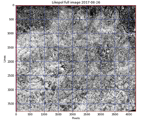
raster=img_like.GetRasterBand(bandnbr).ReadAsArray()
fig, ax = plt.subplots(figsize=(8,8))
ax.set_title('Likepol full image {}'
             .format(tindex[bandnbr-1].date()))
ax.imshow(raster,cmap='gray',vmin=np.nanpercentile(raster,5),vmax=np.nanpercentile(raster,95))
ax.grid(color='blue')
ax.set_xlabel('Pixels')
ax.set_ylabel('Lines')
# plot the subset as rectangle
if subset != None:
    _=ax.add_patch(patches.Rectangle((subset[0],subset[1]),
                                     subset[2],subset[3],
                                     fill=False,edgecolor='red',
                                     linewidth=3))

MAKE THE RGB like/cross/ratio Image

We make an RGB stack to display the like,cross, and ratio data as a color composite.
like、cross、ratioのデータをカラー合成で表示するためにRGBスタックを作ります。

like, cross, ratioというワードはここで初めて出てきました。
以下それぞれ説明します。

• Like
  「同極」または「同位相」データ、すなわち、送信および受信の偏波が同じ場合のデータです。例えば、水平偏波を送信し、水平偏波を受信する場合（HH）、または垂直偏波を送信し、垂直偏波を受信する場合（VV）などが含まれます。このデータは、ターゲットの構造に関する情報を提供することが多いです。

• Cross
  「交差偏波」または「クロス偏波」データ、すなわち、送信偏波と受信偏波が異なる場合のデータです。例えば、水平偏波を送信し、垂直偏波を受信する場合（HV）、またはその逆（VH）などが含まれます。交差偏波データは、ターゲットの形状や表面特性に関する情報を提供することが多いです。

• Ratio
  「比」データ、すなわち、同極偏波と交差偏波のデータの比率を計算することを意味します。比データは、ターゲットの物理特性やダイナミクスを強調するために使用されることがあります。具体的には、HH/VV の比や HV/HH の比などが考えられます。

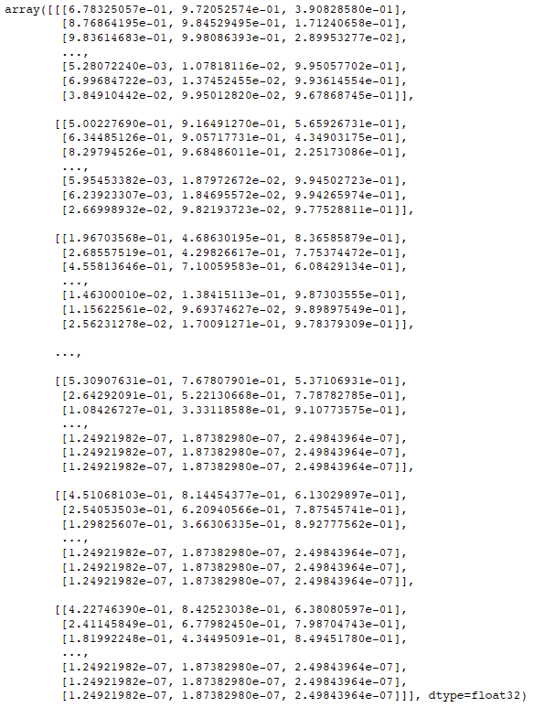
raster_like=img_like.GetRasterBand(bandnbr).ReadAsArray(*subset)
raster_cross=img_cross.GetRasterBand(bandnbr).ReadAsArray(*subset)
rgb,bandnames,sartype=dualpol2rgb(raster_like,raster_cross)

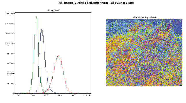
We are interested in displaying the image enhanced with histogram equalization. We can use the function exposure.equalize_hist() from the skimage.exposure module

ヒストグラム均等化で強調された画像を表示てみます。
skimage.exposureモジュールの関数 exposure.equalize_hist() を使います。

rgb_stretched=np.ndarray.astype(rgb.copy(),'float32')
# For each band we apply the strech
for i in range(rgb_stretched.shape[2]):
    rgb_stretched[:,:,i] = np.ndarray.astype(exposure.equalize_hist(rgb_stretched[:,:,i],
    mask=~np.equal(rgb_stretched[:,:,i],0)),'float32')

rgb_stretched

RGB画像に対して各バンド（R、G、B）ごとにヒストグラム平坦化を適用しています。
詳細は以下です。

• RGB画像のコピーと型変換
  • 元のRGB画像 rgb のコピーを作成し、その型を float32 に変換します。このステップは、後続の処理で浮動小数点演算を行うために必要です。
• 各バンドに対するヒストグラム平坦化の適用
  • xposure.equalize_hist を使用してヒストグラム平坦化を適用します
  • mask=~np.equal(rgb_stretched[:,:,i],0) によって、ゼロでないピクセルだけを対象にします。
    結果を float32 型に変換して、元の画像配列に代入します。

Now let's display the the histograms and equalized image side by side.

ヒストグラムと平均化画像を並べて表示してみましょう。

fig,ax = plt.subplots(1,2,figsize=(16,8))
fig.suptitle('Multi-temporal Sentinel-1 backscatter image R:{} G:{} B:{}'
             .format(bandnames[0],bandnames[1],bandnames[2]))
plt.axis('off')
ax[0].hist(rgb[:,:,0].flatten(),histtype='step',color='red',bins=100,range=(0,10000))
ax[0].hist(rgb[:,:,1].flatten(),histtype='step',color='green',bins=100,range=(0,10000))
ax[0].hist(rgb[:,:,2].flatten(),histtype='step',color='blue',bins=100,range=(0,10000))
ax[0].set_title('Histograms')
ax[1].imshow(rgb_stretched)
ax[1].set_title('Histogram Equalized')
_=ax[1].axis('off')

Write the images to an output file

Determine output geometry

First, we need to set the correct geotransformation and projection information. We retrieve the values from the input images and adjust by the subset:

まず、正しいジオトランスフォームと投影情報を設定する必要があります。
入力画像から値を取得し、サブセットによって調整します。

proj=img_like.GetProjection()
geotrans=list(img_like.GetGeoTransform())

subset_xoff=geotrans[0]+subset[0]*geotrans[1]  
subset_yoff=geotrans[3]+subset[1]*geotrans[5] 
geotrans[0]=subset_xoff
geotrans[3]=subset_yoff
geotrans=tuple(geotrans)
geotrans

Convert to 16bit Amplitude image

We use the root of the time series data stack name and append a ts_metrics.tif ending as filenames

時系列データのスタック名を使用し、ts_metrics.tifをファイル名として付加します。

Build a like/cross/ratio amplitude scaled GeoTIFF images

RGB画像の各バンドに対して any2amp 関数を適用し、その結果を新しいGeoTIFFファイルに保存する処理を行っています。

outbands=[]
for i in range(3):
    outbands.append(any2amp(rgb[:,:,i]))

imagename=imagefile_like.replace('_vv_','_lcr_').replace('.vrt','_{}.tif'.format(dates[bandnbr-1].rstrip()))
bandnames=['Like','Cross','Ratio']
Array=np.array(outbands)
CreateGeoTiff(imagename,Array,gdal.GDT_UInt16,0,bandnames,GeoT=geotrans,Projection=proj)

まとめ

本記事では「SAR Handbook」の3章のトレーニングPart6について写経し、自分なりに理解してみました。
どちらかというと自分のための備忘録として記載しましたが、SARについて勉強し始めたところですので、もし間違っている点等ありましたらコメントいただけると幸いです。