導入
最近は、衛星画像の利用が進んでおり、Google Earth Engineのように衛星画像解析が可能なプラットフォームがあります。土地被覆分類などの解析が簡単に実行できますが、ローカルで土地被覆分類しなければならない場合もあります (自分で機械学習モデルを構築する場合、インターネット環境がない場合など)。
この記事ではpythonを用いた土地被覆分類を実装してみます。
環境
Windows 11
python 3.11.9
QGIS 3.40
excel
データ
衛星画像
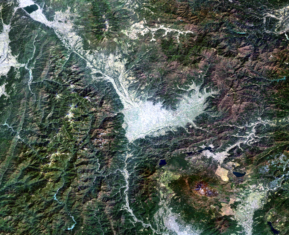
Google Earth Engienを用いて2020年のLandsat 5, 7, 8の合成画像を入手
バンドはNDVI, Tasseled Cap Wetness (TCW), Greenness (TCG), Brightness (TCB), Red (R), Green (G), Blue (B)の順で入ってます。
下の画像は理由もなく選択された山梨県の一部地域。
機械学習モデル
RandomForest (RF)とXGBoostの二つを採用します。
学習データ/検証データ
QGISを用いて点地物を作成し、その地点のピクセルの値を取得
土地被覆は以下の通り設定しました。
0:針葉樹林
1:広葉樹林
2:農地・草原
3:都市
4:水域
5:裸地
実装
0. 必要ライブラリのimport
以下のライブラリを用います。バージョンは気にしていません。
import pandas as pd
import numpy as np
import rasterio
import geopandas as gpd
import matplotlib.pyplot as plt
import optuna
import statistics

from sklearn.feature_selection import SelectKBest, f_classif
from rasterstats import point_query
from sklearn.model_selection import StratifiedKFold, cross_val_score
from sklearn.ensemble import RandomForestClassifier
from xgboost import XGBClassifier
from scipy import ndimage
from tqdm import tqdm
1.学習データ作成
機械学習モデルを構築するために使用する学習/検証データを作成します。
QGISで作成した点地物を用いて、特徴量を取得します。
point_path = "your_path/point.shp"
landsat_path = "/your_path/landsat.tif"
output_path = "/your_path/training_data.shp"

# point_query(point_shp_path, tif_path, band = 1)
# ポイントの位置情報と重なった地点のラスタの値を取得する
point = gpd.read_file(point_path)
point["NDVI"] = point_query(point_path, landsat_path, band = 1)
point["TCW"] = point_query(point_path, landsat_path, band = 2)
point["TCG"] = point_query(point_path, landsat_path, band = 3)
point["TCB"] = point_query(point_path, landsat_path, band = 4)
point["R"] = point_query(point_path, landsat_path, band = 5)
point["G"] = point_query(point_path, landsat_path, band = 6)
point["B"] = point_query(point_path, landsat_path, band = 7)
point.to_file(output_path)
これで出力した学習データを用います。
2.特徴量選択
RFとXGBoostは入力された特徴量の重要度を計算し、自動で特徴量を選択するそうですが、私は実際の中身を見てみたい気持ちがあります。
そこで、各土地被覆と特徴量の関係を分散分析 (ANOVA)を実施してデータの中身を確認してから決めます。
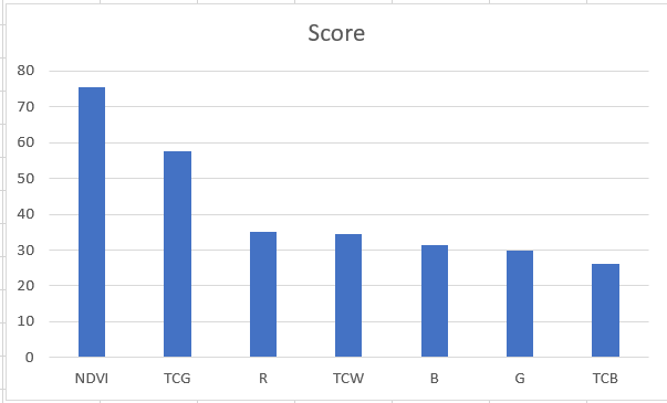
ANOVAの結果のスコアは以下の通り。値が大きいほど、土地被覆と特徴量の間に違いがあることを示しています。この内容に従うと、NDVI、TCGはモデルに組み込んでもよさそうですが、それら以外には大きな差がありません。
個人的にはRはNDVIと関連するところがあるため除いて、水分に関連するTCWは入れたいです。
そこで、NDVI+TCGモデルとNDVI+TCG+TCWモデルの二つを組んでみます。
3.ハイパーパラメータのチューニング
今回はoptunaを用いて、RFとXGBoostのハイパーパラメータをチューニングします。
train_dat = gpd.read_file("your_path/train_data.shp")

feature1 = ["NDVI", "TCG"]
feature2 = ["NDVI", "TCG", "TCW"]

x1, x2, y = train_dat[feature1], train_dat[feature2], train_dat["id"]

kf = StratifiedKFold(n_splits=3, shuffle=True, random_state=1)

##########################################
def xgb_bayse_objective_feature1(trial):
    xgb = XGBClassifier(booster = "gbtree",
                        objective ="multi:softmax",
                        random_state = 42,
                        n_estimators = 10000)
    params = {
        'learning_rate': trial.suggest_float('learning_rate', 0.01, 0.1, log=True),
        'min_child_weight': trial.suggest_int('min_child_weight', 1, 8),
        'max_depth': trial.suggest_int('max_depth', 1, 10),
        'colsample_bytree': trial.suggest_float('colsample_bytree', 0.1, 1.0),
        'subsample': trial.suggest_float('subsample', 0.2, 0.8),
        'reg_alpha': trial.suggest_float('reg_alpha', 0.001, 0.01, log=True),
        'reg_lambda': trial.suggest_float('reg_lambda', 0.001, 0.1, log=True),
        'gamma': trial.suggest_float('gamma', 0.0001, 0.01, log=True),
    }
    xgb.set_params(**params)
    scores = cross_val_score(xgb, x1, y, cv=kf, scoring="neg_log_loss", n_jobs=1)
    val = scores.mean()
    return val

def xgb_bayse_objective_feature2(trial):
    xgb = XGBClassifier(booster = "gbtree",
                        objective ="multi:softmax",
                        random_state = 42,
                        n_estimators = 10000)
    params = {
        'learning_rate': trial.suggest_float('learning_rate', 0.01, 0.1, log=True),
        'min_child_weight': trial.suggest_int('min_child_weight', 1, 8),
        'max_depth': trial.suggest_int('max_depth', 1, 10),
        'colsample_bytree': trial.suggest_float('colsample_bytree', 0.1, 1.0),
        'subsample': trial.suggest_float('subsample', 0.2, 0.8),
        'reg_alpha': trial.suggest_float('reg_alpha', 0.001, 0.01, log=True),
        'reg_lambda': trial.suggest_float('reg_lambda', 0.001, 0.1, log=True),
        'gamma': trial.suggest_float('gamma', 0.0001, 0.01, log=True),
    }
    xgb.set_params(**params)
    scores = cross_val_score(xgb, x2, y, cv=kf, scoring="neg_log_loss", n_jobs=1)
    val = scores.mean()
    return val

def rf_bayse_objective_feature1(trial):
    rf = RandomForestClassifier(criterion="entropy", n_estimators = 1000)
    params = {
        "max_depth":trial.suggest_int("max_depth", 1, 10),
        "min_samples_split":trial.suggest_float("min_samples_split", 0.0, 1.0),
        "min_samples_leaf":trial.suggest_float("min_samples_leaf", 0.0, 1.0)
    }
    rf.set_params(**params)
    scores = cross_val_score(rf, x1, y, cv = kf, scoring="neg_log_loss", n_jobs=1)
    val = scores.mean()
    return val

def rf_bayse_objective_feature2(trial):
    rf = RandomForestClassifier(criterion="entropy", n_estimators = 1000)
    params = {
        "max_depth":trial.suggest_int("max_depth", 1, 10),
        "min_samples_split":trial.suggest_float("min_samples_split", 0.0, 1.0),
        "min_samples_leaf":trial.suggest_float("min_samples_leaf", 0.0, 1.0)
    }
    rf.set_params(**params)
    scores = cross_val_score(rf, x2, y, cv = kf, scoring="neg_log_loss", n_jobs=1)
    val = scores.mean()
    return val
###################################################

trials = 100
print("RF Start")
print(f"Bands is {feature1}")
rf_study = optuna.create_study(direction="maximize", sampler = optuna.samplers.TPESampler(seed = 42))
rf_study.optimize(rf_bayse_objective_feature1, n_trials=trials)
best_params = rf_study.best_trial.params
best_score = rf_study.best_trial.value
print("########################################################")
print(f'{best_params}\nスコア {best_score}')
print("########################################################")

print("***************************************************************")
print("XGBoost Start")
print(f"Bands is {feature1}")
xgb_study = optuna.create_study(direction="maximize", sampler = optuna.samplers.TPESampler(seed = 42))
xgb_study.optimize(xgb_bayse_objective_feature1, n_trials=trials)
best_params = xgb_study.best_trial.params
best_score = xgb_study.best_trial.value
print("########################################################")
print(f'{best_params}\nスコア {best_score}')
print("########################################################")

print("RF Start")
print(f"Bands is {feature2}")
rf_study = optuna.create_study(direction="maximize", sampler = optuna.samplers.TPESampler(seed = 42))
rf_study.optimize(rf_bayse_objective_feature2, n_trials=trials)
best_params = rf_study.best_trial.params
best_score = rf_study.best_trial.value
print("########################################################")
print(f'{best_params}\nスコア {best_score}')
print("########################################################")

print("***************************************************************")
print("XGBoost Start")
print(f"Bands is {feature2}")
xgb_study = optuna.create_study(direction="maximize", sampler = optuna.samplers.TPESampler(seed = 42))
xgb_study.optimize(xgb_bayse_objective_feature2, n_trials=trials)
best_params = xgb_study.best_trial.params
best_score = xgb_study.best_trial.value
print("########################################################")
print(f'{best_params}\nスコア {best_score}')
print("########################################################")
結果は以下のようになりました。
XGBoost
[NDVI, TCG]
{'learning_rate': 0.010935310324903975,
'min_child_weight': 4,
'max_depth': 7,
'colsample_bytree': 0.9606978100500185,
'subsample': 0.3897308128073823,
'reg_alpha': 0.008373191345711269,
'reg_lambda': 0.04577800618991312,
'gamma': 0.004154100253104841}
スコア -1.2335402850732076

[NDVI, TCG, TCW]
{'learning_rate': 0.011134401475562088,
'min_child_weight': 5,
'max_depth': 1,
'colsample_bytree': 0.8361149503592502,
'subsample': 0.5808936682369711,
'reg_alpha': 0.008043212206173432,
'reg_lambda': 0.004175376029789515,
'gamma': 0.008243295071940071}
スコア -1.0390752145327615

RF
[NDVI, TCG]
{'max_depth': 9,
'min_samples_split': 0.033618389988886284,
'min_samples_leaf': 0.027680735584186884}
スコア -1.1454433921770528

[NDVI, TCG, TCW]
{'max_depth': 9,
'min_samples_split': 0.0018600831464722634,
'min_samples_leaf': 0.0203543487201498}
スコア -0.8225644772802955
スコアは大きい方がいいため、NDVI+TCG+TCWのほうがXGBoostとRF共に高い
4.土地被覆分類の実行
次に得られたモデルを用いて土地被覆分類を行います。
output_path = "your_path"

feature1 = ["NDVI", "TCG"] #Band1, Band3
feature2 = ["NDVI", "TCG", "TCW"] # Band1, Band3, Band2

train_dat = gpd.read_file("your_path/Training_Dataset.shp")
train_x1, train_x2, y = train_dat[feature1], train_dat[feature2], train_dat["id"]

tif = rasterio.open("your_path/Landsat.tif")
metadata = tif.meta # 土地被覆分類図出力用
ndvi = tif.read(1)
tcg = tif.read(3)
tcw = tif.read(2)

# 各モデルの特徴量を含むテーブルデータを作成
feature1_vess = []
feature2_vess = []
print(f"Make Data")
for i in range(ndvi.shape[0]):
    for j in range(ndvi.shape[1]):
        # array.shape -> [bands, height, width]
        n = ndvi[i, j]
        tg = tcg[i, j]
        tw = tcw[i, j]

        feature1_vess.append([i, j, n, tg]) # iとjは土地被覆分類図を作成する際に使用する
        feature2_vess.append([i, j, n, tg, tw])

feature1_df = pd.DataFrame(feature1_vess, columns=["i", "j", "NDVI", "TCG"])
feature1_df = feature1_df.dropna()
x1 = feature1_df[feature1].values

feature2_df = pd.DataFrame(feature2_vess, columns=["i", "j", "NDVI", "TCG", "TCW"])
feature2_df = feature2_df.dropna()
x2 = feature2_df[feature2].values

############################################################
# Model Build
print(f"Predict")
xgb_feature1_params ={'learning_rate': 0.010935310324903975,
                      'min_child_weight': 4,
                      'max_depth': 7,
                      'colsample_bytree': 0.9606978100500185,
                      'subsample': 0.3897308128073823,
                      'reg_alpha': 0.008373191345711269,
                      'reg_lambda': 0.04577800618991312,
                      'gamma': 0.004154100253104841}
xgb_feature1 = XGBClassifier(booster='gbtree', objective='multi:softmax', random_state=42, n_estimators=10000,)
xgb_feature1.set_params(**xgb_feature1_params)
xgb_feature1.fit(train_x1, y, verbose = True)

xgb_feature2_params ={'learning_rate': 0.011134401475562088,
                      'min_child_weight': 5,
                      'max_depth': 1,
                      'colsample_bytree': 0.8361149503592502,
                      'subsample': 0.5808936682369711,
                      'reg_alpha': 0.008043212206173432,
                      'reg_lambda': 0.004175376029789515,
                      'gamma': 0.008243295071940071}
xgb_feature2 = XGBClassifier(booster='gbtree', objective='multi:softmax', random_state=42, n_estimators=10000,)
xgb_feature2.set_params(**xgb_feature2_params)
xgb_feature2.fit(train_x2, y, verbose = True)

rf_feature1_params ={'max_depth': 9, 'min_samples_split': 0.033618389988886284, 'min_samples_leaf': 0.027680735584186884}
rf_feature1 = RandomForestClassifier(criterion="entropy", n_estimators=1000)
rf_feature1.set_params(**rf_feature1_params)
rf_feature1.fit(train_x1, y)

rf_feature2_params = {'max_depth': 9, 'min_samples_split': 0.0018600831464722634, 'min_samples_leaf': 0.0203543487201498}
rf_feature2 = RandomForestClassifier(criterion="entropy", n_estimators=1000)
rf_feature2.set_params(**rf_feature2_params)
rf_feature2.fit(train_x2, y)

############################################################
# Predict
feature1_df["Pred_XGB"] = xgb_feature1.predict(x1)
feature2_df["Pred_XGB"] = xgb_feature2.predict(x2)

feature1_df["Pred_RF"] = rf_feature1.predict(x1)
feature2_df["Pred_RF"] = rf_feature2.predict(x2)

# Save Result
print(f"Write")
xgb1_vess = np.full((ndvi.shape[0], ndvi.shape[1]), -1)
xgb2_vess = np.full((ndvi.shape[0], ndvi.shape[1]), -1)
rf1_vess = np.full((ndvi.shape[0], ndvi.shape[1]), -1)
rf2_vess = np.full((ndvi.shape[0], ndvi.shape[1]), -1)

for i, j, xp1, xp2, rp1, rp2 in zip(feature1_df['i'], feature1_df["j"], feature1_df["Pred_XGB"], feature2_df["Pred_XGB"], feature1_df["Pred_RF"], feature2_df["Pred_RF"]):
    xgb1_vess[i, j] = xp1
    xgb2_vess[i, j] = xp2
    rf1_vess[i, j] = rp1
    rf2_vess[i, j] = rp2

def save_raster(array, meta, output):
    new_raster = rasterio.open(output, "w", **meta)
    new_raster.write(array, 1)
    new_raster.close()
    return

print(f"Save")
save_raster(xgb1_vess, metadata, output_path+"/XGBoost_NDVI_TCG.tif")
save_raster(xgb2_vess, metadata, output_path+"/XGBoost_NDVI_TCG_TCW.tif")
save_raster(rf1_vess, metadata, output_path+"/RF_NDVI_TCG.tif")
save_raster(rf2_vess, metadata, output_path+"/RF_NDVI_TCG_TCW.tif")
各土地被覆分類図が以下のようになります。
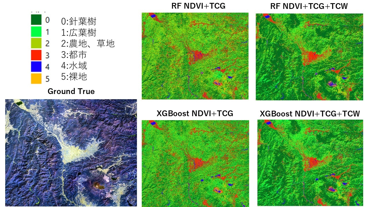
TCWを入力にした方が針葉樹林と広葉樹の分類が上手くできてそうな感じがします。
では、後処理を一度挟んでから精度検証を行いましょう。
5.後処理
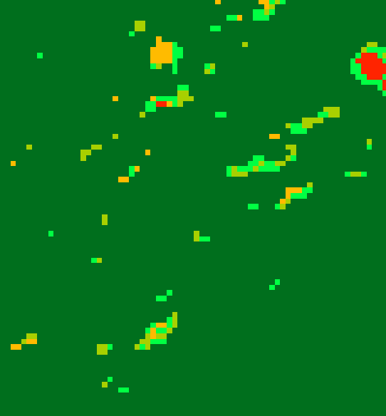
土地被覆分類を行う際に欠かせないのが後処理です。
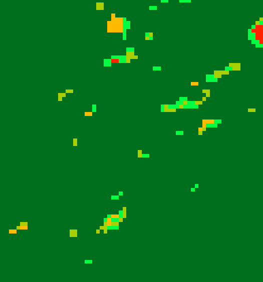
ゴマ塩ノイズ (Salt and Paper Noise)が特に厄介です(下の画像のようなもの)。

土地被覆が1種類だけなら、1を0に、0を1にするだけで除去できますが今回は複数クラスなため、少々工夫する必要があります。
この記事では、ゴマ塩ノイズを周辺の土地被覆情報を用いて除去していきます。
def postprocess(tif_path, output_path):
    tif = rasterio.open(tif_path)
    metadata = tif.meta
    array = tif.read(1) # band 1の読み込み
    labels = np.unique(array)

    for l in labels:
        mask = np.where(array == l, 1, 0) # 対象ラベルを1、それ以外を0とする
        s = ndimage.generate_binary_structure(2, 2)
        patch_mask, patch_num = ndimage.label(mask, s)
        patch_unique, patch_size = np.unique(patch_mask, return_counts = True)
        patch_arr = np.array([patch_unique, patch_size]).T
        noises = patch_arr[patch_arr[:, 1] == 1]

        with tqdm(total = mask.shape[0]) as pbar:
            for i in range(mask.shape[0]):
                pbar.set_description(f"label: {l}")
                for j in range(mask.shape[1]):

                    # あるピクセルの場所はゴマ塩ノイズであるかを判定
                    # 判定がTrueなら、周辺ピクセルの最頻値に置き換え
                    if np.any(noises == patch_mask[i, j]):
                        vess.append([i, j, patch_mask[i, j], l])

                        # ラスタの四隅である場合
                        if (i == 0)&(j == 0):
                            p1, p2, p3 = array[i, j+1], array[i+1,j+1], array[i+1, j]
                            array[i, j] = statistics.mode([p1, p2, p3])
                        elif (i == array.shape[0]-1)&(j == array.shape[1]-1):
                            p1, p2, p3 = array[i, j-1], array[i-1,j-1], array[i-1, j]
                            array[i, j] = statistics.mode([p1, p2, p3])
                        elif (i == 0)&(j == array.shape[1]-1):
                            p1, p2, p3 = array[i-1, j], array[i+1,j-1], array[i+1, j]
                            array[i, j] = statistics.mode([p1, p2, p3])
                        elif (i == array.shape[0]-1)&(j == 0):
                            p1, p2, p3 = array[i-1, j], array[i-1,j+1], array[i, j+1]
                            array[i, j] = statistics.mode([p1, p2, p3])

                        # もし、ラスタの端のラインなら
                        elif (i == 0)&(j != 0)&(j != array.shape[1]-1):
                            p1, p2, p3, p4, p5 = array[i, j-1], array[i,j+1], array[i+1, j-1], array[i+1, j], array[i+1, j+1]
                            array[i, j] = statistics.mode([p1, p2, p3, p4, p5])
                        elif (i == array.shape[0]-1)&(j != 0)&(j != array.shape[1]-1):
                            p1, p2, p3, p4, p5 = array[i, j-1], array[i,j+1], array[i-1, j-1], array[i-1, j], array[i-1, j+1]
                            array[i, j] = statistics.mode([p1, p2, p3, p4, p5])
                        elif (i != 0)&(i != array.shape[0-1])&(j == 0):
                            p1, p2, p3, p4, p5 = array[i-1, j], array[i+1,j], array[i-1, j+1], array[i, j+1], array[i+1, j+1]
                            array[i, j] = statistics.mode([p1, p2, p3, p4, p5])
                        elif (i != 0)&(i != array.shape[0]-1)&(j == array.shape[1]-1):
                            p1, p2, p3, p4, p5 = array[i-1, j], array[i+1,j], array[i-1, j-1], array[i, j-1], array[i+1, j-1]
                            array[i, j] = statistics.mode([p1, p2, p3, p4, p5])

                        # それ以外の場所
                        else:
                            p1, p2, p3, p4, p5, p6, p7, p8 = array[i-1, j-1], array[i-1,j], array[i-1, j+1], array[i, j-1], array[i, j+1], array[i+1, j-1], array[i+1, j], array[i+1, j+1]
                            array[i, j] = statistics.mode([p1, p2, p3, p4, p5, p6, p7, p8])

                pbar.update(1)

    new_raster = rasterio.open(output_path, "w", **metadata)
    new_raster.write(array, 1)
    new_raster.close()
    return

tif_path = "your_path/RF_NDVI_TCG.tif"
output_path ="your_path/RF_NDVI_TCG_postprocessed.tif"
postprocess(tif_path, output_path)

tif_path = "your_path/RF_NDVI_TCG_TCW.tif"
output_path ="your_path/RF_NDVI_TCG_TCW_postprocessed.tif"
postprocess(tif_path, output_path)

tif_path = "your_path/XGBoost_NDVI_TCG.tif"
output_path ="your_path/XGBoost_NDVI_TCG_postprocessed.tif"
postprocess(tif_path, output_path)

tif_path = "your_path/XGBoost_NDVI_TCG_TCW.tif"
output_path ="your_path/XGBoost_NDVI_TCG_TCW_postprocessed.tif"
postprocess(tif_path, output_path)
このコードを実行すると、以下のようなに1ピクセルのみを周辺の最頻値のクラスに置換できます。
6.精度検証
最後に精度検証を行います。
まず、検証用データの作成を行います。目視で作成した学習データと同様の点地物を用います。
検証データの点数は60点×各土地被覆で計360個です。
point_path = "your_path/val_points.shp"
output_path = "your_path/Validation_Dataset_labels.xlsx"

point = gpd.read_file(point_path)

lulc_path = "your_path/RF_NDVI_TCG_postprocessed.tif"
# interpolate='nearest'にすることで、点直下の値をそのまま取得できる
point["RF_NDVI_TCG"] = point_query(point_path, lulc_path, band = 1, interpolate='nearest')

lulc_path = "your_path/RF_NDVI_TCG_TCW_postprocessed.tif"
point = gpd.read_file(point_path)
point["RF_NDVI_TCG_TCW"] = point_query(point_path, lulc_path, band = 1, interpolate='nearest')

lulc_path = "your_path/XGBoost_NDVI_TCG_postprocessed.tif"
point = gpd.read_file(point_path)
point["XGB_NDVI_TCG"] = point_query(point_path, lulc_path, band = 1, interpolate='nearest')

lulc_path = "your_path/XGBoost_NDVI_TCG_TCW_postprocessed.tif"
point = gpd.read_file(point_path)
point["XGB_NDVI_TCG_TCW"] = point_query(point_path, lulc_path, band = 1, interpolate='nearest')

point.to_excel(output_path)
出力したexcelファイルを用いてクロス集計表を作成します。
今回の精度指標は User's Accuracy (UA) と Producer's Accuracy (PA) と Overall Accuracy (OA) の三つです。
それぞれの指標の概要は以下です。
UA: 土地被覆図の分類がどれだけの割合で実際を表現しているか (予測->実際)
PA: 地上の地物の再現率 (実際->予測)
OA: 全体の精度
以下に混合行列の結果をまとめます。
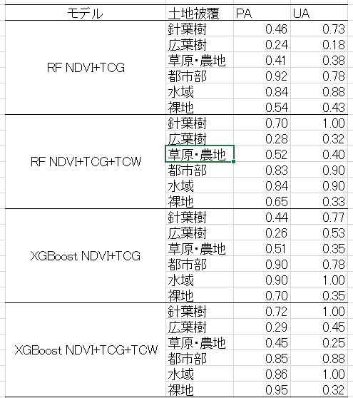

TCWを追加することで概ね全体の精度が向上しています。
NDVI+TCG+TCWのRFとXGBoostを比較した場合、得意・不得意があることが分かります。裸地が特に顕著ですが、全体的にはXGBoostのほうが優れているようです。
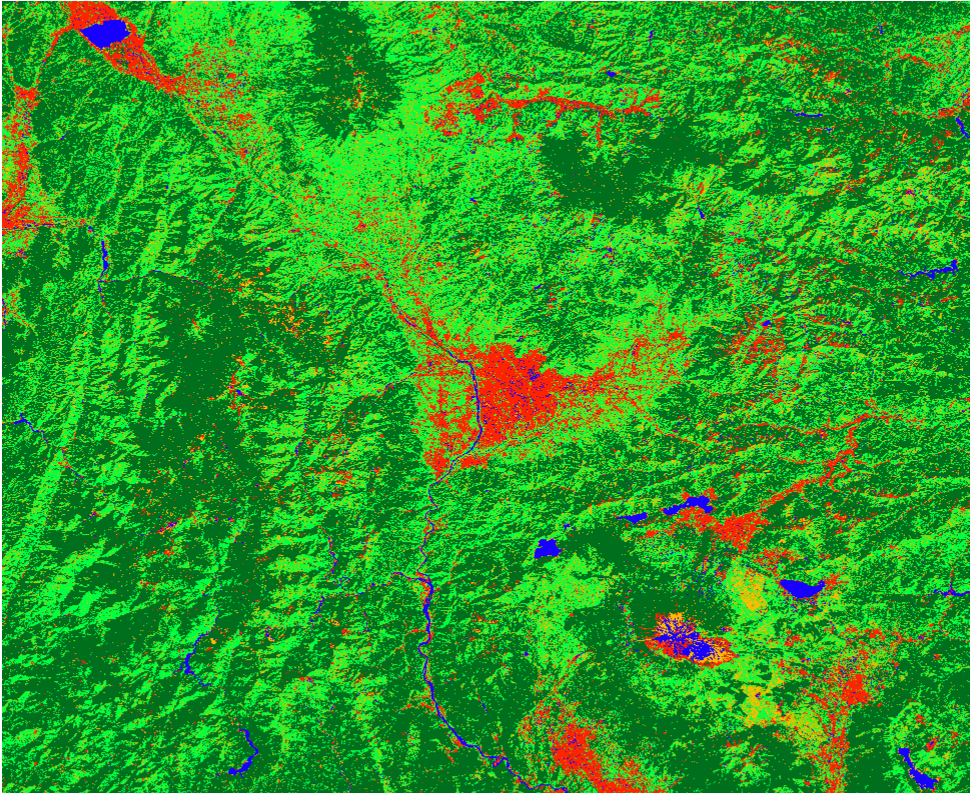
最後にXGBoostの精度が良かったNDVI+TCG+TCWの最終出力結果を表示します。
おわりに
今回はローカル環境で機械学習を用いた土地被覆分類を行いました。
ANOVAを用いた特徴量選択やハイパーパラメータのチューニングにも挑戦してみましたが、やはり直感を大切にしたいです。
まだまだ勉強すべきことが多いです。
次回の記事ですが、今回使用したデータを用いて土地被覆分類におけるゼネラリストV.S.スペシャリストに挑戦します。
それでは。