はじめに
今回、SIGNATEの『【練習問題】レンタル自転車の利用者予測』に取り組みました。機械学習については、学びたてでまだ多くのことができていない状況ですが、コンペなどを通じて少しずつ成長していければなぁと思っています。
コンペの内容
下記の練習問題に取り組みました。
【練習問題】レンタル自転車の利用者数予測
2年間の季節情報や気象情報から、各日の1時間ごとのレンタル自転車の利用者数を予測するこのモデルを作成していただきます
実際のコード
1.データの読み込み
# ライブラリのインポート
import numpy as np
import pandas as pd
import matplotlib.pyplot as plt
%matplotlib inline
# ファイルの読み込み・表示
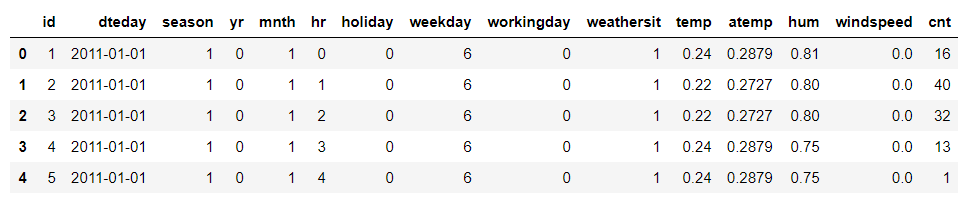
train = pd.read_csv('train.tsv',sep='\t')
test = pd.read_csv('test.tsv',sep='\t')
train.head()
2.データ内容の把握
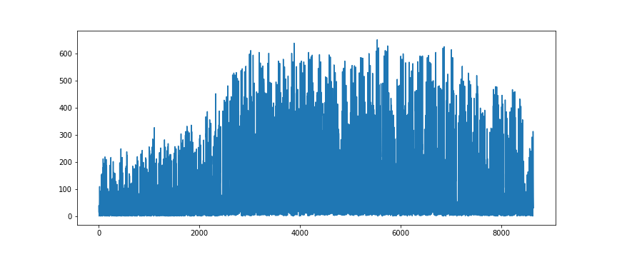
# 利用状況をプロットしてみる
plt.figure(figsize=(12,5))
plt.plot(train['id'],train['cnt'])
# 試しにとある1週間の利用状況をプロット
# 1.日付ごとに変数に格納
_day0703 = train.query('dteday == "2011-07-03"')# 日
_day0704 = train.query('dteday == "2011-07-04"')# 月
_day0705 = train.query('dteday == "2011-07-05"')# 火
_day0706 = train.query('dteday == "2011-07-06"')# 水
_day0707 = train.query('dteday == "2011-07-07"')# 木
_day0708 = train.query('dteday == "2011-07-08"')# 金
_day0709 = train.query('dteday == "2011-07-09"')# 土
# 2.各日付をグラフ表示
plt.figure(figsize=(12,5))
plt.plot(_day0703['hr'],_day0703['cnt'],label='Sun')
plt.plot(_day0704['hr'],_day0704['cnt'],label='Mon')
plt.plot(_day0705['hr'],_day0705['cnt'],label='Tue')
plt.plot(_day0706['hr'],_day0706['cnt'],label='Wed')
plt.plot(_day0707['hr'],_day0707['cnt'],label='Thu')
plt.plot(_day0708['hr'],_day0708['cnt'],label='Fri')
plt.plot(_day0709['hr'],_day0709['cnt'],label='Sat')
plt.legend()
plt.grid()
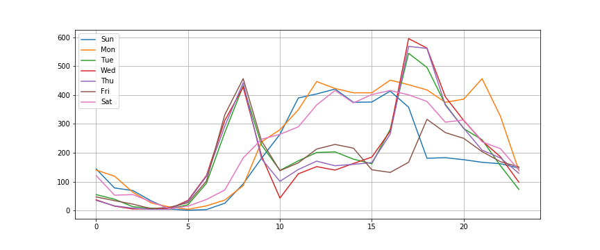
・休日と平日で利用状況が異なるらしい。
・平日では、午前6~10時、午後16~21時が多く利用されているため、通勤・通学などに用いられてそう。
休日、また時間帯によって利用状況が変化するため、線形回帰は不向きと考えXGBoostを選択。
3.XGBoostを使った学習
# XGBoostのライブラリのインポート
import xgboost as xgb
from sklearn.model_selection import GridSearchCV
from sklearn.metrics import mean_squared_error
# xgboostモデルの作成
reg = xgb.XGBRegressor()
# id2500以前は、傾向が違うため、カット(運用開始など?)
train = train[train['id'] > 2500]
# 説明変数、目的変数を格納
X_train = train.drop(['id','dteday','cnt'], axis=1)
y_train = train['cnt']
X_test = test.drop(['id','dteday'], axis=1)
# ハイパーパラメータ探索
reg_cv = GridSearchCV(reg, {'max_depth': [2,4,6], 'n_estimators': [50,100,200]}, verbose=1)
reg_cv.fit(X_train, y_train)
print(reg_cv.best_params_, reg_cv.best_score_)
# 改めて最適パラメータで学習
reg = xgb.XGBRegressor(**reg_cv.best_params_)
reg.fit(X_train, y_train)
4.モデルの確認
# 学習データを使って予測
pred_train = reg.predict(X_train)
# 予測値が妥当か確認
train_value = y_train.values
_df = pd.DataFrame({'actual':train_value,'pred':pred_train})
_df.plot(figsize=(12,5))
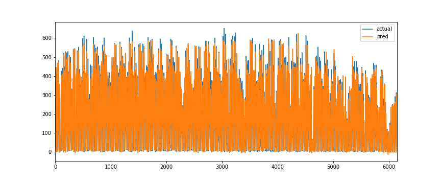
おおむね、正しく予測できていそう。
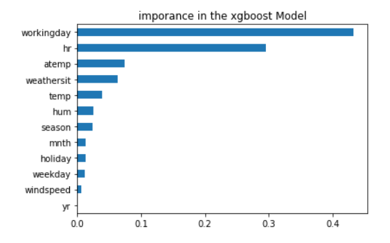
5.評特徴量の重要度を確認
# feature importance のプロット
importances = pd.Series(reg.feature_importances_, index = X_train.columns)
importances = importances.sort_values()
importances.plot(kind = "barh")
plt.title("imporance in the xgboost Model")
plt.show()
6.提出ファイルの作成
# テストデータに対し予測値の算出
pred_test = reg.predict(X_test)
# 結果を張り付け、ファイル出力
sample = pd.read_csv("sample_submit.csv",header=None)
sample[1] = pred_test
sample.to_csv("submit01.csv",index=None,header=None)
結果&まとめ
209人中29位でした。
今回は、単純にXGBoostに入れただけなので、他にも特徴量を作り上げたり、別の学習モデルやアンサンブル学習など、いろいろ工夫する余地がありそうです。
また再チャレンジできたらと思っているので、その時にはまた記事にしたいと思います。