初めに
今後使いそうなメソッドのまとめ。
- pandas バージョン
- 1.0.5
前回と同様最高気温の月平均を用いる。
max_temperature.csv
年,1月,2月,3月,4月,5月,6月,7月,8月,9月,10月,11月,12月,年の値
1876,6.6,8.2,13.6,17.5,21.7,22.8,28.6,31.6,26.8,20.4,15.8,11.0,18.7
1877,8.8,8.8,11.3,19.1,21.5,26.0,31.0,30.5,25.8,21.3,14.4,10.2,19.1
1878,7.2,7.1,12.9,16.2,22.7,24.1,29.8,28.5,26.3,20.2,14.1,10.9,18.3
1879,9.0,10.9,13.0,17.1,21.9,25.2,30.4,31.1,25.4,19.4,15.7,14.0,19.4
1880,8.8,10.1,13.8,16.7,22.6,23.9,28.0,29.5,27.0,21.6,16.8,11.1,19.2
・・・
import pandas as pd

df = pd.read_csv('max_temperature.csv', index_col='年')
print(df)
        1月    2月    3月    4月    5月    6月    7月    8月    9月   10月   11月   12月   年の値
年
1876   6.6   8.2  13.6  17.5  21.7  22.8  28.6  31.6  26.8  20.4  15.8  11.0  18.7
1877   8.8   8.8  11.3  19.1  21.5  26.0  31.0  30.5  25.8  21.3  14.4  10.2  19.1
1878   7.2   7.1  12.9  16.2  22.7  24.1  29.8  28.5  26.3  20.2  14.1  10.9  18.3
1879   9.0  10.9  13.0  17.1  21.9  25.2  30.4  31.1  25.4  19.4  15.7  14.0  19.4
1880   8.8  10.1  13.8  16.7  22.6  23.9  28.0  29.5  27.0  21.6  16.8  11.1  19.2
...    ...   ...   ...   ...   ...   ...   ...   ...   ...   ...   ...   ...   ...
2016  10.6  12.2  14.9  20.3  25.2  26.3  29.7  31.6  27.7  22.6  15.5  13.8  20.9
2017  10.8  12.1  13.4  19.9  25.1  26.4  31.8  30.4  26.8  20.1  16.6  11.1  20.4
2018   9.4  10.1  16.9  22.1  24.6  26.6  32.7  32.5  26.6  23.0  17.7  12.1  21.2
2019  10.3  11.6  15.4  19.0  25.3  25.8  27.5  32.8  29.4  23.3  17.7  12.6  20.9
2020  11.1  13.3  16.0  18.2  24.0  27.5  27.7  34.1  28.1  21.4  18.6  12.3  21.0

[145 rows x 13 columns]
メソッド
add
print(df + 1000)
          1月      2月      3月      4月      5月      6月      7月      8月      9月     10月     11月     12月     年の値
年
1876  1006.6  1008.2  1013.6  1017.5  1021.7  1022.8  1028.6  1031.6  1026.8  1020.4  1015.8  1011.0  1018.7
1877  1008.8  1008.8  1011.3  1019.1  1021.5  1026.0  1031.0  1030.5  1025.8  1021.3  1014.4  1010.2  1019.1
1878  1007.2  1007.1  1012.9  1016.2  1022.7  1024.1  1029.8  1028.5  1026.3  1020.2  1014.1  1010.9  1018.3
1879  1009.0  1010.9  1013.0  1017.1  1021.9  1025.2  1030.4  1031.1  1025.4  1019.4  1015.7  1014.0  1019.4
1880  1008.8  1010.1  1013.8  1016.7  1022.6  1023.9  1028.0  1029.5  1027.0  1021.6  1016.8  1011.1  1019.2
...      ...     ...     ...     ...     ...     ...     ...     ...     ...     ...     ...     ...     ...
2016  1010.6  1012.2  1014.9  1020.3  1025.2  1026.3  1029.7  1031.6  1027.7  1022.6  1015.5  1013.8  1020.9
2017  1010.8  1012.1  1013.4  1019.9  1025.1  1026.4  1031.8  1030.4  1026.8  1020.1  1016.6  1011.1  1020.4
2018  1009.4  1010.1  1016.9  1022.1  1024.6  1026.6  1032.7  1032.5  1026.6  1023.0  1017.7  1012.1  1021.2
2019  1010.3  1011.6  1015.4  1019.0  1025.3  1025.8  1027.5  1032.8  1029.4  1023.3  1017.7  1012.6  1020.9
2020  1011.1  1013.3  1016.0  1018.2  1024.0  1027.5  1027.7  1034.1  1028.1  1021.4  1018.6  1012.3  1021.0

[145 rows x 13 columns]
add_prefix
シリーズの場合、行名には接頭辞が付きます。DataFrameの場合、列名には接頭辞が付きます。
print('type(df.dtypes): {}\n'.format(type(df.dtypes)))

# シリーズの場合行ラベルに接頭辞が追加される
print(df.dtypes.add_prefix('列: '))
type(df.dtypes): <class 'pandas.core.series.Series'>

列: 1月     float64
列: 2月     float64
列: 3月     float64
列: 4月     float64
列: 5月     float64
列: 6月     float64
列: 7月     float64
列: 8月     float64
列: 9月     float64
列: 10月    float64
列: 11月    float64
列: 12月    float64
列: 年の値    float64
dtype: object
# DataFrameの場合列名に接頭辞が追加される
print(df.add_prefix('列: '))
      列: 1月  列: 2月  列: 3月  列: 4月  列: 5月  列: 6月  列: 7月  列: 8月  列: 9月  列: 10月  列: 11月  列: 12月  列: 年の値
年
1876    6.6    8.2   13.6   17.5   21.7   22.8   28.6   31.6   26.8    20.4    15.8    11.0    18.7
1877    8.8    8.8   11.3   19.1   21.5   26.0   31.0   30.5   25.8    21.3    14.4    10.2    19.1
1878    7.2    7.1   12.9   16.2   22.7   24.1   29.8   28.5   26.3    20.2    14.1    10.9    18.3
1879    9.0   10.9   13.0   17.1   21.9   25.2   30.4   31.1   25.4    19.4    15.7    14.0    19.4
1880    8.8   10.1   13.8   16.7   22.6   23.9   28.0   29.5   27.0    21.6    16.8    11.1    19.2
...     ...    ...    ...    ...    ...    ...    ...    ...    ...     ...     ...     ...     ...
2016   10.6   12.2   14.9   20.3   25.2   26.3   29.7   31.6   27.7    22.6    15.5    13.8    20.9
2017   10.8   12.1   13.4   19.9   25.1   26.4   31.8   30.4   26.8    20.1    16.6    11.1    20.4
2018    9.4   10.1   16.9   22.1   24.6   26.6   32.7   32.5   26.6    23.0    17.7    12.1    21.2
2019   10.3   11.6   15.4   19.0   25.3   25.8   27.5   32.8   29.4    23.3    17.7    12.6    20.9
2020   11.1   13.3   16.0   18.2   24.0   27.5   27.7   34.1   28.1    21.4    18.6    12.3    21.0

[145 rows x 13 columns]
# インデックスの更新
df.index = ['西暦' + str(i) + '年' for i in range(1876, 2021)]
print(df)
           1月    2月    3月    4月    5月    6月    7月    8月    9月   10月   11月   12月   年の値
西暦1876年   6.6   8.2  13.6  17.5  21.7  22.8  28.6  31.6  26.8  20.4  15.8  11.0  18.7
西暦1877年   8.8   8.8  11.3  19.1  21.5  26.0  31.0  30.5  25.8  21.3  14.4  10.2  19.1
西暦1878年   7.2   7.1  12.9  16.2  22.7  24.1  29.8  28.5  26.3  20.2  14.1  10.9  18.3
西暦1879年   9.0  10.9  13.0  17.1  21.9  25.2  30.4  31.1  25.4  19.4  15.7  14.0  19.4
西暦1880年   8.8  10.1  13.8  16.7  22.6  23.9  28.0  29.5  27.0  21.6  16.8  11.1  19.2
...       ...   ...   ...   ...   ...   ...   ...   ...   ...   ...   ...   ...   ...
西暦2016年  10.6  12.2  14.9  20.3  25.2  26.3  29.7  31.6  27.7  22.6  15.5  13.8  20.9
西暦2017年  10.8  12.1  13.4  19.9  25.1  26.4  31.8  30.4  26.8  20.1  16.6  11.1  20.4
西暦2018年   9.4  10.1  16.9  22.1  24.6  26.6  32.7  32.5  26.6  23.0  17.7  12.1  21.2
西暦2019年  10.3  11.6  15.4  19.0  25.3  25.8  27.5  32.8  29.4  23.3  17.7  12.6  20.9
西暦2020年  11.1  13.3  16.0  18.2  24.0  27.5  27.7  34.1  28.1  21.4  18.6  12.3  21.0

[145 rows x 13 columns]
apply
axis{0 or ‘index’, 1 or ‘columns’}, default 0
0 または 'index' : 各列に関数を適用します。
1 または 'columns':各行に関数を適用します。
# 各列に対して和を計算する
print(df.apply(np.sum, axis=0))
1月     1313.3
2月     1381.6
3月     1835.3
4月     2620.0
5月     3220.4
6月     3636.9
7月     4195.4
8月     4432.5
9月     3863.9
10月    3061.9
11月    2358.0
12月    1674.2
年の値    2800.2
dtype: float64
# 各行に対して和を計算する
print(df.apply(np.sum, axis=1))
年
1876    243.3
1877    247.8
1878    238.3
1879    252.5
1880    249.1
        ...
2016    271.3
2017    264.9
2018    275.5
2019    271.6
2020    273.3
Length: 145, dtype: float64
# 各要素に対して平方根をとる
print(df.apply(np.sqrt))
            1月        2月        3月        4月        5月        6月        7月        8月        9月       10月       11月       12月       年の値
年
1876  2.569047  2.863564  3.687818  4.183300  4.658326  4.774935  5.347897  5.621388  5.176872  4.516636  3.974921  3.316625  4.324350
1877  2.966479  2.966479  3.361547  4.370355  4.636809  5.099020  5.567764  5.522681  5.079370  4.615192  3.794733  3.193744  4.370355
1878  2.683282  2.664583  3.591657  4.024922  4.764452  4.909175  5.458938  5.338539  5.128353  4.494441  3.754997  3.301515  4.277850
1879  3.000000  3.301515  3.605551  4.135215  4.679744  5.019960  5.513620  5.576737  5.039841  4.404543  3.962323  3.741657  4.404543
1880  2.966479  3.178050  3.714835  4.086563  4.753946  4.888763  5.291503  5.431390  5.196152  4.647580  4.098780  3.331666  4.381780
...        ...       ...       ...       ...       ...       ...       ...       ...       ...       ...       ...       ...       ...
2016  3.255764  3.492850  3.860052  4.505552  5.019960  5.128353  5.449771  5.621388  5.263079  4.753946  3.937004  3.714835  4.571652
2017  3.286335  3.478505  3.660601  4.460942  5.009990  5.138093  5.639149  5.513620  5.176872  4.483302  4.074310  3.331666  4.516636
2018  3.065942  3.178050  4.110961  4.701064  4.959839  5.157519  5.718391  5.700877  5.157519  4.795832  4.207137  3.478505  4.604346
2019  3.209361  3.405877  3.924283  4.358899  5.029911  5.079370  5.244044  5.727128  5.422177  4.827007  4.207137  3.549648  4.571652
2020  3.331666  3.646917  4.000000  4.266146  4.898979  5.244044  5.263079  5.839521  5.300943  4.626013  4.312772  3.507136  4.582576

[145 rows x 13 columns]
agg
指定された軸上で1つ以上の操作を使用して集計します。
# 列ごとに和を計算、最小値を取得
print(df.agg(['sum', 'min']))
         1月      2月      3月      4月      5月      6月      7月      8月      9月     10月     11月     12月     年の値
sum  1313.3  1381.6  1835.3  2620.0  3220.4  3636.9  4195.4  4432.5  3863.9  3061.9  2358.0  1674.2  2800.2
min     5.5     5.8     9.6    14.8    19.2    21.6    25.1    25.7    23.2    18.5    12.9     8.7    17.5
# "1 月" 列と "2 月" 列で異なる処理をする
# "1 月" 列では max 処理をしていないので NaN の値が表示される
print(df.agg({'1月': ['sum', 'min'], '2月': ['min', 'max'], '3月': ['mean']}))
          1月    2月         3月
max      NaN  13.3        NaN
mean     NaN   NaN  12.657241
min      5.5   5.8        NaN
sum   1313.3   NaN        NaN
# axis="columns" は行ごとに、各列の値の処理をする
# axis=1でも同じ結果を得る
df.agg("mean", axis="columns")
年
1876    18.715385
1877    19.061538
1878    18.330769
1879    19.423077
1880    19.161538
          ...
2016    20.869231
2017    20.376923
2018    21.192308
2019    20.892308
2020    21.023077
Length: 145, dtype: float64
assign
DataFrameに新しい列を割り当てます。
# すべての行、インデックス 0 からインデックス 11 までの列( 1 月 ~ 12 月 )を抽出し、各行に対して和を計算する
# その和を "SUM" という新たな列として割り当てる
df = df.assign(SUM=df.iloc[:, 0:12].apply(np.sum, axis=1))
print('add column "SUM":\n{}\n'.format(df))
add column "SUM":
        1月    2月    3月    4月    5月    6月    7月    8月    9月   10月   11月   12月   年の値    SUM
年
1876   6.6   8.2  13.6  17.5  21.7  22.8  28.6  31.6  26.8  20.4  15.8  11.0  18.7  224.6
1877   8.8   8.8  11.3  19.1  21.5  26.0  31.0  30.5  25.8  21.3  14.4  10.2  19.1  228.7
1878   7.2   7.1  12.9  16.2  22.7  24.1  29.8  28.5  26.3  20.2  14.1  10.9  18.3  220.0
1879   9.0  10.9  13.0  17.1  21.9  25.2  30.4  31.1  25.4  19.4  15.7  14.0  19.4  233.1
1880   8.8  10.1  13.8  16.7  22.6  23.9  28.0  29.5  27.0  21.6  16.8  11.1  19.2  229.9
...    ...   ...   ...   ...   ...   ...   ...   ...   ...   ...   ...   ...   ...    ...
2016  10.6  12.2  14.9  20.3  25.2  26.3  29.7  31.6  27.7  22.6  15.5  13.8  20.9  250.4
2017  10.8  12.1  13.4  19.9  25.1  26.4  31.8  30.4  26.8  20.1  16.6  11.1  20.4  244.5
2018   9.4  10.1  16.9  22.1  24.6  26.6  32.7  32.5  26.6  23.0  17.7  12.1  21.2  254.3
2019  10.3  11.6  15.4  19.0  25.3  25.8  27.5  32.8  29.4  23.3  17.7  12.6  20.9  250.7
2020  11.1  13.3  16.0  18.2  24.0  27.5  27.7  34.1  28.1  21.4  18.6  12.3  21.0  252.3

[145 rows x 14 columns]
# 各行の "SUM" 列の値に対し 12 で割った値を新たに "MEAN" 列として割り当てる
df = df.assign(MEAN=df['SUM'] / 12)
print('add column "MEAN":\n{}\n'.format(df))
add column "MEAN":
        1月    2月    3月    4月    5月    6月    7月    8月    9月   10月   11月   12月   年の値    SUM       MEAN
年
1876   6.6   8.2  13.6  17.5  21.7  22.8  28.6  31.6  26.8  20.4  15.8  11.0  18.7  224.6  18.716667
1877   8.8   8.8  11.3  19.1  21.5  26.0  31.0  30.5  25.8  21.3  14.4  10.2  19.1  228.7  19.058333
1878   7.2   7.1  12.9  16.2  22.7  24.1  29.8  28.5  26.3  20.2  14.1  10.9  18.3  220.0  18.333333
1879   9.0  10.9  13.0  17.1  21.9  25.2  30.4  31.1  25.4  19.4  15.7  14.0  19.4  233.1  19.425000
1880   8.8  10.1  13.8  16.7  22.6  23.9  28.0  29.5  27.0  21.6  16.8  11.1  19.2  229.9  19.158333
...    ...   ...   ...   ...   ...   ...   ...   ...   ...   ...   ...   ...   ...    ...        ...
2016  10.6  12.2  14.9  20.3  25.2  26.3  29.7  31.6  27.7  22.6  15.5  13.8  20.9  250.4  20.866667
2017  10.8  12.1  13.4  19.9  25.1  26.4  31.8  30.4  26.8  20.1  16.6  11.1  20.4  244.5  20.375000
2018   9.4  10.1  16.9  22.1  24.6  26.6  32.7  32.5  26.6  23.0  17.7  12.1  21.2  254.3  21.191667
2019  10.3  11.6  15.4  19.0  25.3  25.8  27.5  32.8  29.4  23.3  17.7  12.6  20.9  250.7  20.891667
2020  11.1  13.3  16.0  18.2  24.0  27.5  27.7  34.1  28.1  21.4  18.6  12.3  21.0  252.3  21.025000

[145 rows x 15 columns]
# 各行(axis=1)の中央値を新たに "MEDIAN" 列として割り当てる
df = df.assign(MEDIAN=df.iloc[:, 0:12].median(axis=1))
print('add column "MEDIAN":\n{}\n'.format(df))
add column "MEDIAN":
        1月    2月    3月    4月    5月    6月    7月    8月    9月   10月   11月   12月   年の値    SUM       MEAN  MEDIAN
年
1876   6.6   8.2  13.6  17.5  21.7  22.8  28.6  31.6  26.8  20.4  15.8  11.0  18.7  224.6  18.716667   18.95
1877   8.8   8.8  11.3  19.1  21.5  26.0  31.0  30.5  25.8  21.3  14.4  10.2  19.1  228.7  19.058333   20.20
1878   7.2   7.1  12.9  16.2  22.7  24.1  29.8  28.5  26.3  20.2  14.1  10.9  18.3  220.0  18.333333   18.20
1879   9.0  10.9  13.0  17.1  21.9  25.2  30.4  31.1  25.4  19.4  15.7  14.0  19.4  233.1  19.425000   18.25
1880   8.8  10.1  13.8  16.7  22.6  23.9  28.0  29.5  27.0  21.6  16.8  11.1  19.2  229.9  19.158333   19.20
...    ...   ...   ...   ...   ...   ...   ...   ...   ...   ...   ...   ...   ...    ...        ...     ...
2016  10.6  12.2  14.9  20.3  25.2  26.3  29.7  31.6  27.7  22.6  15.5  13.8  20.9  250.4  20.866667   21.45
2017  10.8  12.1  13.4  19.9  25.1  26.4  31.8  30.4  26.8  20.1  16.6  11.1  20.4  244.5  20.375000   20.00
2018   9.4  10.1  16.9  22.1  24.6  26.6  32.7  32.5  26.6  23.0  17.7  12.1  21.2  254.3  21.191667   22.55
2019  10.3  11.6  15.4  19.0  25.3  25.8  27.5  32.8  29.4  23.3  17.7  12.6  20.9  250.7  20.891667   21.15
2020  11.1  13.3  16.0  18.2  24.0  27.5  27.7  34.1  28.1  21.4  18.6  12.3  21.0  252.3  21.025000   20.00
count
各列または行について、NA以外のセルをカウントします。
# 1876 年 1 月 を NaN という値に更新する
df.loc[1876, '1月'] = np.nan

# 1876 年以降 2 月のすべての値を NaN という値に更新する
df.loc[df.index > 1875, '2月'] = np.nan
print('df:\n{}\n'.format(df))
df:
        1月  2月    3月    4月    5月    6月    7月    8月    9月   10月   11月   12月   年の値
年
1876   NaN NaN  13.6  17.5  21.7  22.8  28.6  31.6  26.8  20.4  15.8  11.0  18.7
1877   8.8 NaN  11.3  19.1  21.5  26.0  31.0  30.5  25.8  21.3  14.4  10.2  19.1
1878   7.2 NaN  12.9  16.2  22.7  24.1  29.8  28.5  26.3  20.2  14.1  10.9  18.3
1879   9.0 NaN  13.0  17.1  21.9  25.2  30.4  31.1  25.4  19.4  15.7  14.0  19.4
1880   8.8 NaN  13.8  16.7  22.6  23.9  28.0  29.5  27.0  21.6  16.8  11.1  19.2
...    ...  ..   ...   ...   ...   ...   ...   ...   ...   ...   ...   ...   ...
2016  10.6 NaN  14.9  20.3  25.2  26.3  29.7  31.6  27.7  22.6  15.5  13.8  20.9
2017  10.8 NaN  13.4  19.9  25.1  26.4  31.8  30.4  26.8  20.1  16.6  11.1  20.4
2018   9.4 NaN  16.9  22.1  24.6  26.6  32.7  32.5  26.6  23.0  17.7  12.1  21.2
2019  10.3 NaN  15.4  19.0  25.3  25.8  27.5  32.8  29.4  23.3  17.7  12.6  20.9
2020  11.1 NaN  16.0  18.2  24.0  27.5  27.7  34.1  28.1  21.4  18.6  12.3  21.0

[145 rows x 13 columns]
# 列ごとに、各行に含まれる NaN 以外の要素の個数をカウント
print('df.count():\n{}\n'.format(df.count()))
df.count():
1月     144
2月       0
3月     145
4月     145
5月     145
6月     145
7月     145
8月     145
9月     145
10月    145
11月    145
12月    145
年の値    145
dtype: int64
# 行ごとに、各列に含まれる NaN 以外の要素の個数をカウント
print("df.count(axis='columns'):\n{}\n".format(df.count(axis='columns')))
df.count(axis='columns'):
年
1876    11
1877    12
1878    12
1879    12
1880    12
        ..
2016    12
2017    12
2018    12
2019    12
2020    12
Length: 145, dtype: int64
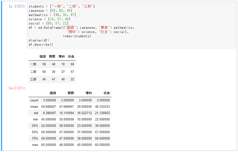
describe
記述統計を生成します。
記述統計には、NaN値を除いて、データセットの分布の中心傾向、分散、および形状を要約した統計が含まれます。
students = ['一郎', '二郎', '三郎']
japanese = [59, 60, 45]
mathmatics = [48, 30, 47]
science = [10, 37, 40]
social = [60, 57, 22]
df = pd.DataFrame({'国語': japanese, '算数': mathmatics,
                    '理科': science, '社会': social},
                  index=students)
print(df)
df.describe()
filter
指定されたインデックスラベルに従って、行または列を抽出します。
print(df.filter(items=['1月', '12月'], axis=1))
        1月   12月
年
1876   6.6  11.0
1877   8.8  10.2
1878   7.2  10.9
1879   9.0  14.0
1880   8.8  11.1
...    ...   ...
2016  10.6  13.8
2017  10.8  11.1
2018   9.4  12.1
2019  10.3  12.6
2020  11.1  12.3

[145 rows x 2 columns]
# 正規表現を使い、4 月 ~ 6 月の列を抽出
print(df.filter(regex='^[4-6]', axis=1))
        4月    5月    6月
年
1876  17.5  21.7  22.8
1877  19.1  21.5  26.0
1878  16.2  22.7  24.1
1879  17.1  21.9  25.2
1880  16.7  22.6  23.9
...    ...   ...   ...
2016  20.3  25.2  26.3
2017  19.9  25.1  26.4
2018  22.1  24.6  26.6
2019  19.0  25.3  25.8
2020  18.2  24.0  27.5

[145 rows x 3 columns]
# 西暦に "88" が並ぶ行であり、かつ 4 月 ~ 6 月の列を抽出
print(df.filter(like='88', axis=0).filter(regex='^[4-6]', axis=1))
        4月    5月    6月
年
1880  16.7  22.6  23.9
1881  16.9  22.5  25.6
1882  18.4  21.9  24.0
1883  16.6  19.9  23.6
1884  16.2  20.2  23.6
1885  14.8  19.3  23.4
1886  16.9  20.3  25.1
1887  17.3  19.2  24.1
1888  17.5  20.4  22.8
1889  16.3  20.3  25.0
1988  18.1  22.1  25.5
groupby
groupby操作では、オブジェクトを分割し、関数を適用し、結果を結合します。これは、大量のデータをグループ化し、これらのグループに対する操作を計算するために使用できます。
df = pd.DataFrame({'教科': ['国語', '算数', '算数', '理科', '理科', '社会', '国語'],
                   '点数': [50, 49, 62, 53, 32, 43, 64]})
print(df)
   教科  点数
0  国語  50
1  算数  49
2  算数  62
3  理科  53
4  理科  32
5  社会  43
6  国語  64
# "教科" 列の重複をまとめる
# .mean() により平均を取りながらまとめる
print(df.groupby(['教科']).mean())
      点数
教科
国語  57.0
理科  42.5
社会  43.0
算数  55.5
import pandas as pd
arrays = [['一郎', '一郎', '二郎', '二郎'],
          ['国語', '算数', '国語', '算数']]
index = pd.MultiIndex.from_arrays(arrays, names=('名前', '教科'))
df = pd.DataFrame({'点数': [53, 28, 40, 39]},
                  index=index)
print(df)

# 各生徒の平均点をテーブルにする
print(df.groupby(level=0).mean())

# 各教科の平均点をテーブルにする
print(df.groupby(level=1).mean())
       点数
名前 教科
一郎 国語  53
     算数  28
二郎 国語  40
     算数  39

      点数
名前
一郎  40.5
二郎  39.5

      点数
教科
国語  46.5
算数  33.5
idxmax
要求された軸上の最大値のインデックスのうち、最初に出現したインデックスを返します。
students = ['一郎', '二郎', '三郎']
# 国語の点数
japanese = [59, 60, 45]
# 数学の点数
mathmatics = [48, 30, 47]
# 理科の点数
science = [10, 37, 40]
# 社会の点数
social = [60, 57, 22]
df = pd.DataFrame({'国語': japanese, '数学': mathmatics,
                    '理科': science, '社会': social},
                  index=students)
print('df:\n{}\n'.format(df))

# 各教科の最高点を取った生徒のテーブル
print('df.idxmax():\n{}\n'.format(df.idxmax()))

# 各生徒の最高点を取った教科のテーブル
print('df.idxmax():\n{}\n'.format(df.idxmax(axis=1)))
df:
    国語  数学  理科  社会
一郎  59  48  10  60
二郎  60  30  37  57
三郎  45  47  40  22

df.idxmax():
国語    二郎
数学    一郎
理科    三郎
社会    一郎
dtype: object

df.idxmax():
一郎    社会
二郎    国語
三郎    数学
dtype: object
info
# 列ごとの情報を表示する
print(df.info(verbose=True))
print('------------------------')
# 列ごとの情報は出力しない
print(df.info(verbose=False))
<class 'pandas.core.frame.DataFrame'>
Index: 3 entries, 一郎 to 三郎
Data columns (total 4 columns):
国語    3 non-null int64
数学    3 non-null int64
理科    3 non-null int64
社会    3 non-null int64
dtypes: int64(4)
memory usage: 120.0+ bytes
None
------------------------
<class 'pandas.core.frame.DataFrame'>
Index: 3 entries, 一郎 to 三郎
Columns: 4 entries, 国語 to 社会
dtypes: int64(4)
memory usage: 120.0+ bytes
None
insert
指定した場所のDataFrameに列を挿入します。
students = ['一郎', '二郎', '三郎']
japanese = [59, 60, 45]
mathmatics = [48, 30, 47]
science = [10, 37, 40]
social = [60, 57, 22]
df = pd.DataFrame({'国語': japanese, '数学': mathmatics,
                    '理科': science, '社会': social},
                  index=students)
print('df:\n{}\n'.format(df))

# 最初の列(loc=0)に体育を追加
df.insert(loc=0, column='体育', value=[65, 12, 58])
print('insert 体育:\n{}\n'.format(df))
df:
    国語  数学  理科  社会
一郎  59  48  10  60
二郎  60  30  37  57
三郎  45  47  40  22

insert 体育:
    体育  国語  数学  理科  社会
一郎  65  59  48  10  60
二郎  12  60  30  37  57
三郎  58  45  47  40  22
isin
DataFrameの各要素が値に含まれているかどうかを示します。
students = ['一郎', '二郎', '三郎']
like_subject = ['算数', '社会', '理科']
unlike_subject = ['国語', '理科', '算数']
df = pd.DataFrame({'好きな教科': like_subject, '嫌いな教科': unlike_subject},
                  index=students)
print('df:\n{}\n'.format(df))
# 好きまたは嫌いな強化に"算数"が含まれているか
print(df.isin(['算数']))
# 好きな教科に"算数"が含まれているか
print(df.isin({'好きな教科': ['算数']}))
# 嫌いな教科に"理科"が含まれているか
print(df.isin({'嫌いな教科': ['理科']}))
df:
   好きな教科 嫌いな教科
一郎    算数    国語
二郎    社会    理科
三郎    理科    算数

    好きな教科  嫌いな教科
一郎   True  False
二郎  False  False
三郎  False   True
    好きな教科  嫌いな教科
一郎   True  False
二郎  False  False
三郎  False  False
    好きな教科  嫌いな教科
一郎  False  False
二郎  False   True
三郎  False  False
items
DataFrame列を反復処理し、列名とコンテンツを含むタプルをシリーズとして返します。
subjects = ['国語', '算数', '理科', '社会']
score = [65, 45, 36, 64]
mean = [50.46, 58.90, 42.15, 68.96]
df = pd.DataFrame({'点数': score, '平均点': mean},
                  index=subjects)
print(f'df: \n{df}\n')

print('---items example---')
for label, content in df.items():
    print(f'label: {label}')
    print(f'content: \n{content}')
df:
    点数    平均点
国語  65  50.46
算数  45  58.90
理科  36  42.15
社会  64  68.96

---items example---
label: 点数
content:
国語    65
算数    45
理科    36
社会    64
Name: 点数, dtype: int64
label: 平均点
content:
国語    50.46
算数    58.90
理科    42.15
社会    68.96
Name: 平均点, dtype: float64
rename
行/列名を変更します。
students = ['一郎', '二郎', '三郎']
japanese = [59, 60, 45]
mathmatics = [48, 30, 47]
science = [10, 37, 40]
social = [60, 57, 22]
df = pd.DataFrame({'国語': japanese, '算数': mathmatics,
                    '理科': science, '社会': social},
                  index=students)
print('df:\n{}\n'.format(df))
df = df.rename(columns={"国語": "japanese", "算数": "mathmatics",
                        "理科": "science", "社会": "social studies"})
print('rename df:\n{}\n'.format(df))
df:
    国語  算数  理科  社会
一郎  59  48  10  60
二郎  60  30  37  57
三郎  45  47  40  22

rename df:
    japanese  mathmatics  science  social studies
一郎        59          48       10              60
二郎        60          30       37              57
三郎        45          47       40              22
sem
要求された軸の平均の不偏標準誤差を返します。
print(df.sem(axis=1))
print(df.sem(axis=0))
年
1876    2.134180
1877    2.191140
1878    2.135637
1879    1.966520
1880    1.930708
          ...
2016    1.938820
2017    2.025990
2018    2.133177
2019    1.990988
2020    1.944590
Length: 145, dtype: float64
-----------------------
1月     0.108507
2月     0.127538
3月     0.122152
4月     0.104449
5月     0.109502
6月     0.111669
7月     0.147541
8月     0.120107
9月     0.118103
10月    0.089512
11月    0.091009
12月    0.099818
年の値    0.070890
dtype: float64
std
要求された軸のサンプル標準偏差を返します。
print(df.std(axis=1))
print('-----------------------')
print(df.std(axis=0))
年
1876    7.694895
1877    7.900268
1878    7.700150
1879    7.090387
1880    6.961266
          ...
2016    6.990516
2017    7.304810
2018    7.691279
2019    7.178610
2020    7.011319
Length: 145, dtype: float64
-----------------------
1月     1.306594
2月     1.535764
3月     1.470910
4月     1.257727
5月     1.318581
6月     1.344674
7月     1.776632
8月     1.446284
9月     1.422150
10月    1.077872
11月    1.095893
12月    1.201967
年の値    0.853628
dtype: float64
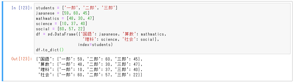
to_dict
DataFrameを辞書に変換します。
students = ['一郎', '二郎', '三郎']
japanese = [59, 60, 45]
mathmatics = [48, 30, 47]
science = [10, 37, 40]
social = [60, 57, 22]
df = pd.DataFrame({'国語': japanese, '算数': mathmatics,
                    '理科': science, '社会': social},
                  index=students)
df.to_dict()
{'国語': {'一郎': 59, '二郎': 60, '三郎': 45},
 '算数': {'一郎': 48, '二郎': 30, '三郎': 47},
 '理科': {'一郎': 10, '二郎': 37, '三郎': 40},
 '社会': {'一郎': 60, '二郎': 57, '三郎': 22}}
transpose
行と列を転置します。
students = ['一郎', '二郎', '三郎']
japanese = [59, 60, 45]
mathmatics = [48, 30, 47]
science = [10, 37, 40]
social = [60, 57, 22]
df = pd.DataFrame({'国語': japanese, '算数': mathmatics,
                    '理科': science, '社会': social},
                  index=students)
print(df)
print('-------------------')
print(df.T)
    国語  算数  理科  社会
一郎  59  48  10  60
二郎  60  30  37  57
三郎  45  47  40  22
-------------------
    一郎  二郎  三郎
国語  59  60  45
算数  48  30  47
理科  10  37  40
社会  60  57  22
var
要求された軸上の不偏分散を返します。
print(df.var(axis=1))
print('-----------------------')
print(df.var(axis=0))
年
1876    59.211410
1877    62.414231
1878    59.292308
1879    50.273590
1880    48.459231
          ...
2016    48.867308
2017    53.360256
2018    59.155769
2019    51.532436
2020    49.158590
Length: 145, dtype: float64
-----------------------
1月     1.707187
2月     2.358570
3月     2.163576
4月     1.581877
5月     1.738656
6月     1.808148
7月     3.156420
8月     2.091739
9月     2.022511
10月    1.161807
11月    1.200982
12月    1.444725
年の値    0.728681
dtype: float64
参考記事