【初心者向け】標本分散(Sample Dispersion)と不偏分散(Unbiased Dispersion)

それにつけても、何故標本分散（Sample Dispersion）sum((x-mean(x)^2))/length(x)の分母はlength(x)で、不偏分散（Unbiased Dispersion）sum((x-mean(x)^2))/(length(x)-1)の分母は(length(x)-1)なのでしょうか？ こういう疑問に突き当たった時は実際にシミュレーションしてみるに限ります。

何故、不偏分散はN-1で割るのか？

分散だけn−1で割るのは、どうも不公平な感じがする、という方がいるかもしれない。試しに、実際のデータで見てみよう。

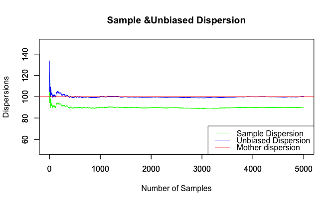
まず、N(50, 10)の乱数を5000ケース発生させ、10ケースで 1サンプルとして標本分散と不偏分散を求める。

次に、サンプルの平均値を求め、グラフ化する。標本分散は母分散100から外れたところを推移し、決して母分散に近づくことはない。

統計言語Rによる検証

Time_code<-seq(1,5000) 
SD0<-NULL #標本分散初期化
UD0<-NULL #不偏分散初期化

#試行の実施

for (i in Time_code){
smp<-rnorm(10,mean=50,sd=10)
#標本分散の算出結果追加
SD0<-c(SD0,sum((smp-mean(smp))^2)/length(smp))
#不偏分散の算出結果追加
UD0<-c(UD0,sum((smp-mean(smp))^2)/(length(smp)-1))
}

#描画データ準備

Sample_Dispersion<-NULL
Unbiased_Dispersion<-NULL
for (i in Time_code){

Sample_Dispersion<-c(Sample_Dispersion,mean(SD0[1:i]))
Unbiased_Dispersion<-c(Unbiased_Dispersion,mean(UD0[1:i]))
}

#グラフ描画

plot(Time_code,Sample_Dispersion,type="l",col=rgb(0,1,0),xlim=c(0,5000),ylim=c(50,150),main="Sample &Unbiased Dispersion",xlab="Number of Samples",ylab="Dispersions")
par(new=T) #上書き
plot(Time_code,Unbiased_Dispersion,type="l",col=rgb(0,0,1),xlim=c(0,5000),ylim=c(50,150),main="",xlab="",ylab="")

#母分散追加

abline(h=100,col=rgb(1,0,0))

#凡例

legend("bottomright", legend=c("Sample Dispersion","Unbiased Dispersion","Mother dispersion"), lty=c(1,1,1), col=c(rgb(0,1,0),rgb(0,0,1),rgb(1,0,0)))

最終結果

Sample_Dispersion[5000]
[1] 90.08727
Unbiased_Dispersion[5000]
[1] 100.097

本当にその通り推移してますね…