Simplex Projectionによる時系列データの予測

はじめに

前回記事 で投稿したEDMについて、学習内容の反芻と時間的外挿に挑戦するため、Simplex ProjectionをPythonで実装したお話です。

提案者であるSugiharaらの研究室で実装されている pyEDM については、入力のDataFrame外の予測に対応していないということで実装する運びとなりました (参考) 。

また本実装については京都大学の潮先生の ブログ を参考にしております。

Simplex Projection

0. データ準備

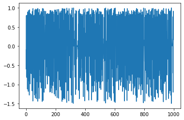
pyEDMのサンプルデータセットから テント写像 のデータを使用します。

!pip install pyEDM

import pyEDM
tentmap = pyEDM.sampleData['TentMap']

print(tentmap.head())

  Time  TentMap
0    1  -0.09920
1    2  -0.60130
2    3   0.79980
3    4  -0.79441
4    5   0.79800

1. Time-delay Embedding

変数 $y_t$ に対して { ${y_{t}, y_{t-\tau}, ..., y_{t-(E-1)\tau} }$ } のように自身のラグを用いて元の動態を再構成します。
実際には対象の変数以外にも、関連する他変数を用いることもできます。
今回は簡単のために1変数で、かつ、$E=2, \tau=1$ とします。
実際は動態の再構成精度に大きく依存する変数なので、事前に手持ちデータに対して推定が必要です。

なおpyEDMの場合は Embed() が用意されています (doc) 。

実装したもの

def time_delay_embedding(objective_df, target_var, E=2, tau=1):
    return_df = pd.DataFrame(objective_df[target_var].values,
                             columns=[target_var+"(t-0)"],
                             index=objective_df.index)    

    for i in range(tau, E*tau-1, tau):
        colname = target_var + "(t-" + str(i) + ")"
        return_df[colname] = objective_df[[target_var]].shift(i)

    return return_df.dropna()

emb_df = time_delay_embedding(tentmap, "TentMap", E=2, tau=1)
print(emb_df.head())

   TentMap(t-0)  TentMap(t-1)
1      -0.60130      -0.09920
2       0.79980      -0.60130
3      -0.79441       0.79980
4       0.79800      -0.79441
5      -0.81954       0.79800

2. Nearest Neighborの探索

今回の実装では手持ちのデータの最新値をターゲットとして、その $1$ 時刻後を予測するものとしています。

target_pt = emb_df.iloc[-1,:].values # 予測の基準となる最新値

diff = emb_df.values - target_pt # 基準点から手持ちデータ全点間の差分
l2_distance = np.linalg.norm(diff, ord=2, axis=1) # 差分からL2ノルムの計算
l2_distance = pd.Series(l2_distance, index=emb_df.index, name="l2") # ソートしたいのでpandas.Seriesに変換

nearest_sort = l2_distance.iloc[:-1].sort_values(ascending=True) # 末尾 (= 基準である最新値) を除いて近い順にソート

print(nearest_sort.head(3))

index    distance
  124    0.003371
  177    0.018171
  163    0.018347
Name: l2

3. Nearest Neighborの動き

予測の基準である点を $y_{t}$ 、抽出した近傍点を { $y_{t_1}, y_{t_2}, y_{t_3} $ } とすると、
{ $y_{t_1+1}, y_{t_2+1}, y_{t_3+1} $ } を用いて予測したい点 $y_{t+1}$ を計算します。
前節で得られた近傍点のインデックスが { 124, 177, 163 } なので、
{ 125, 178, 164 } に該当する点を使用することになります。

参照する近傍点数に制限はありませんが、埋め込み次元 $E$ に対して $E+1$ を採用しています。

knn = int(emb_df.shape[1] + 1)
nn_index = np.array(nearest_sort.iloc[:knn,:].index.tolist())
nn_future_index = nn_index + pt

print(nn_index, "-->", nn_future_index)

nn_future_points = lib_df.loc[nn_future_index].values
print(nn_future_points)

[124 177 163] --> [125 178 164]

[[0.16743 0.91591]
 [0.15932 0.91998]
 [0.1335  0.93295]]

4. 予測点の計算

基準点 $y_{t}$ と { $y_{t_1}, y_{t_2}, y_{t_3} $ } までの距離に応じて、{ $y_{t_1+1}, y_{t_2+1}, y_{t_3+1} $ } に対する重み { $w_{t_1+1}, w_{t_2+1}, w_{t_3+1} $ } を計算します。

nn_distances = nearest_sort.loc[nn_index].values # 基準点からyt1, yt2, yt3までの距離
nn_weights = np.exp(-nn_distances/nn_distances[0]) # 重みを計算
total_weight = np.sum(nn_weights)

print("nn_distances")
print("nn_weights")
print("total_weight")

[0.00337083 0.01817143 0.01834696]
[0.36787944 0.00455838 0.00432709]
0.376764916711149

重みを用いて予測点 $y_{t+1}$ を計算します。
式としては単純な加重平均で、
$ y_{t+1} = \frac{w_{t_1+1} \times y_{t_1+1} + w_{t_2+1} \times y_{t_2+1} + w_{t_3+1} \times y_{t_3+1}}{w_{total}}$

forecast_point = list()
for yt in nn_future_points.T:
    forecast_point.append(np.sum((yt * nn_weights) / total_weight))

print(forecast_point)

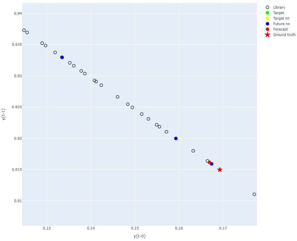
[0.16694219792961462, 0.9161549438807427]

ちなみにこの場合の正解は
ground_truth: [0.16928 0.91498]
となりますので、かなり近い値が求められています。

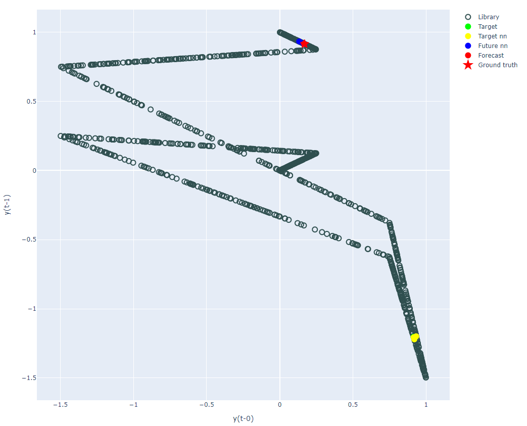
最後に計算の様子をプロットしてみました。

全体図

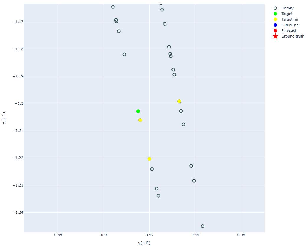
基準点 $y_{t}$ と { $y_{t_1}, y_{t_2}, y_{t_3} $ } の拡大

予測値と真値の拡大

1. ～ 4. を結合した関数全体

2. def forecast_simplex_projection(input_df=None,
                                   forecast_tp=1, knn=None
                                  ):
       if input_df is None:
           raise Exception("Invalid argument: is None: lib_df<pandas.DataFrame> is None")
   
       if knn is None:
           knn = int(input_df.shape[1] + 1) # 埋め込み次元+1
   
       # 入力DataFrameから変数名を取得
       input_cols = input_df.columns.tolist()
   
       # 後段の再帰処理のためにデータをDeepCopy
       lib_df = input_df.copy()
   
       # forecast_tpで指定されたステップまで1ステップ予測を再帰的に実行
       forecast_points = list()
       for pt in range(1, forecast_tp+1):
           # 基準点からライブラリ各点までの距離計算
           target_pt = lib_df.iloc[-1,:].values
           lib_pt = lib_df.values
   
           diff = lib_pt - target_pt
   
           l2_distance = np.linalg.norm(diff, ord=2, axis=1)
           l2_distance = pd.Series(l2_distance, index=lib_df.index, name="l2")
   
           # 距離を近い順にソート
           nearest_sort = l2_distance.iloc[:-1].sort_values(ascending=True)
   
           # 基準点に対する近傍点のインデックスとt+1のインデックス
           nn_index = np.array(nearest_sort.iloc[:knn].index.tolist())
           nn_future_index = nn_index + 1
   
           # 近傍点の距離に応じて重みを計算           
           nn_distances = nearest_sort.loc[nn_index].values
           nn_distances = nn_distances + 1.0e-6
   
           nn_weights = np.exp(-nn_distances/nn_distances[0])
           total_weight = np.sum(nn_weights)
   
           # 埋め込み次元ごとに予測値を計算
           forecast_value = list()
           for yt in nn_future_points.values.T:
               forecast_value.append(np.sum((yt * nn_weights) / total_weight))
   
           # 予測結果をライブラリに追加
           forecast_points.append(forecast_value)
           series_forecast = pd.Series(forecast_value, index=input_df.columns)
           lib_df = lib_df.append(series_forecast, ignore_index=True)
   
       forecast_points = np.array(forecast_points)
   
       return forecast_points
   

終わりに

今回はEDMの中でも最も単純なSimplex ProjectionをPythonで実装しました。
手法としては他にもS-MapやMultiview Embeddingなどが挙げられます。
また、動態の再構成には多変数で異なるラグを使用することも可能で、予測精度に影響します。
次回以降はこういった内容に挑戦していきます。