NISAの取り崩しシミュレーターを作ってみた。

はじめに

　2024年から新NISAが始まり、資産形成のために投資を始めたという方も多くいらっしゃると思います。資産運用の目的は様々ですが、中にはFinancial Independence Retire Early(通称FIRE)を目指している場合もあります。
　筆者もFIREを達成すべく資産形成に励んでいます。そこで気になるのは、どれだけの額をどこに投資し、いくら取り崩すことができるのかということです。
　巷ではS＆P500指数もしくは全世界株に連動する投資信託に全力投資し、年4%ずつ取り崩せば、資金が枯渇することなくFIREすることが可能であるといわれています(4%ルール)。
　年利平均値から考えると成立することが確認できますが、実際のデータを用いた場合の値動きを検証するためのプログラムを作成しました。
※簡単のために取り崩し時の税金は考慮していません。考慮する場合はプログラムを適宜修正してください。

プログラム本体

import yfinance as yf
import pandas as pd
import matplotlib.pyplot as plt


class ETFWithdrawalSimulator:
    def __init__(self, ticker: str, start_date: str, initial_investment: int, monthly_withdrawal_rate: float):
        """
        ETF取り崩しシミュレーションを行うクラス

        Args:
            ticker (str): ETFのティッカー（例: "SPY"）
            start_date (str): データ取得開始日（例: "2000-01-01"）
            initial_investment (int): 初期投資額（例: 30000000）
            monthly_withdrawal_rate (float): 毎月の取り崩し率（例: 0.01）
        """
        self.ticker = ticker
        self.start_date = start_date
        self.initial_investment = initial_investment
        self.monthly_withdrawal_rate = monthly_withdrawal_rate
        self.simulation_result = None
    
    def fetch_data(self):
        """ETFデータを取得し、月次リターンを計算する"""
        data = yf.download(self.ticker, start=self.start_date, progress=False)
        data_monthly = data['Adj Close'].resample('ME').ffill()
        monthly_returns = data_monthly.pct_change().dropna()
        return monthly_returns
    
    def run_simulation(self):
        """シミュレーションを実行する"""
        monthly_returns = self.fetch_data()
        investment = self.initial_investment
        balance_history = []

        for i, return_rate in enumerate(monthly_returns):
            withdrawal_amount = investment * self.monthly_withdrawal_rate
            investment *= (1 + return_rate)
            investment -= withdrawal_amount
            balance_history.append((monthly_returns.index[i], investment, withdrawal_amount))
            if investment <= 0:
                break

        df = pd.DataFrame(balance_history, columns=["Date", "Balance", "Withdrawal"])
        df["Cumulative Withdrawal"] = df["Withdrawal"].cumsum()
        self.simulation_result = df
        return df

    def plot_results(self):
        """シミュレーション結果を可視化する"""
        if self.simulation_result is None:
            raise ValueError("Simulation has not been run yet.")
        
        df = self.simulation_result
        
        # 残高推移
        plt.figure(figsize=(10, 6))
        plt.plot(df["Date"], df["Balance"], label="Balance")
        plt.title(f"{self.ticker} Withdrawal Simulation")
        plt.xlabel("Date")
        plt.ylabel("Balance (JPY)")
        plt.grid()
        plt.legend()
        plt.show()

        # 取り崩し額推移
        plt.figure(figsize=(10, 6))
        plt.plot(df["Date"], df["Withdrawal"], label="Monthly Withdrawal", color="red")
        plt.title(f"{self.ticker} Monthly Withdrawal")
        plt.xlabel("Date")
        plt.ylabel("Withdrawal (JPY)")
        plt.grid()
        plt.legend()
        plt.show()

        # 累計取り崩し額
        plt.figure(figsize=(10, 6))
        plt.plot(df["Date"], df["Cumulative Withdrawal"], label="Cumulative Withdrawal", color="red")
        plt.title(f"{self.ticker} Cumulative Withdrawal")
        plt.xlabel("Date")
        plt.ylabel("Cumulative Withdrawal (JPY)")
        plt.grid()
        plt.legend()
        plt.show()

    def save_results(self, filename="simulation_result.csv"):
        """シミュレーション結果をCSVファイルに保存する"""
        if self.simulation_result is None:
            raise ValueError("Simulation has not been run yet.")
        self.simulation_result.to_csv(filename, index=False)


# シミュレーション条件
ticker = "SPY"  # SP500連動ETF
start_date = "2000-01-01"  # データ取得開始日
initial_investment = 30000000  # 初期投資額（3000万円）
monthly_withdrawal_rate = 0.01  # 毎月取り崩す割合（1%）

# シミュレーションの実行
simulator = ETFWithdrawalSimulator(ticker, start_date, initial_investment, monthly_withdrawal_rate)
simulation_result = simulator.run_simulation()
simulator.plot_results()
simulator.save_results()

シミュレーション条件として

• tickerシンボル
• 取り崩し開始日(FIRE開始日)
• FIRE時の資産額
• 毎月の取り崩し割合

を設定することで、実際のデータを用いてシミュレーションを行うことができます。

一例として以下の条件で実際にシミュレーションした結果を示します。

• 投資対象：SPY
• FIRE開始日：2000年1月1日
• 投資額：3000万
• 毎月の取り崩し割合：0.3%(=4%ルール)

図1. 総資産の推移

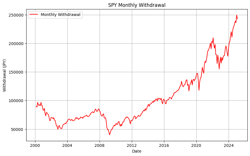
図2. 毎月の取り崩し額の推移

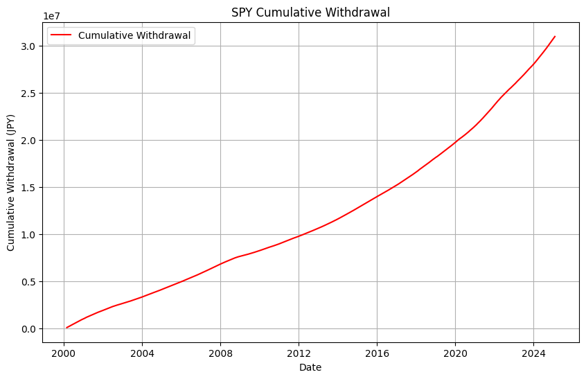
図3. 取り崩し額の総計

これによると、投資額3000万円では毎月の取り崩し額は多くても20万円程度となることがわかりました。またリーマンショック付近では取り崩し額が5万円を割ることもあり、とてもFIREができているとは言えないことがわかりました。

さいごに

今回の例ではSPYを用いましたが、それぞれの投資戦略にあったものを用いてシミュレーションをしてください。投資に絶対はなく、過去にこうであったから未来もこうだとは言い切れません。しかし、このようなシミュレーションを繰り返すことで投資への判断に自信を持つことができるようになり、結果として資産形成の成功につながると思います。
皆様の資産形成がうまくいくことを願っています。

その他のtickerシンボル例

• VTI: 全世界株式
• QQQ: NASDAQ100指数
• QLD: NASDAQ100指数の2倍の値動き(いわゆるレバナス)
• TQQQ: NASDAQ100指数の3倍の値動き