Background

いろいろな判別分析を比較してみた「Rで判別分析いろいろ（11種類+ Deep Learning）」とか「眼鏡っ娘分類システムの改良（判別分析12種類：SVM, Random Forest, Deep Learning 他）」が、毎回チューニングするのに結構時間がかかる。主な原因は３つ

それぞれ違ったパッケージを使っていたので、設定方法が違ったりして調べるのに時間がかかる
グリッドサーチが実装されていない場合は自力実装
並列化とか結構面倒

そこで、すこし前に見つけて、いつかやってみようとおもっていた「caret」

いろいろなパッケージのwapperになっていて、同じ使い勝手でグリッドサーチができるようになっている
並列化も勝手にやってくれる。とてもカンタン
すごくたくさんの手法が使える

Summary

方法

データ・セットは２値分類で、お手軽につかえるkernlabパッケージのspam
トレーニング用とテスト用にデータを分けておく
いろいろな分類手法を、caretでトレーニング＆自動的にチューニングする
テストデータで正解率を計算
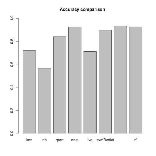
各モデルの正解率を比較する

結果

手法	caretで指定するmethod名	正解率
k Nearest Neighbor	knn	0.725
naive Bayse	nb	0.565
Decision Tree	rpart	0.840
3層ニューラルネット	nnet	0.921
学習ベクトル量子化ニューラルネットワーク	lvq	0.706
Support Vector Machine	svmRadial	0.900
Gradient Boosting Machine	gbm	0.930
Random Forest	rf	0.920

結論

チューニング済のモデルで正解率を計算した。３層ニューラルネット、Gradient Boosting Model, Random Forest、次いでSVMが良かった。
個別のパッケージを使うよりも、コードが圧倒的に見やすい。グリッドサーチを自分で書かなくてよい。自分で並列化しなくてよい。
チューニング結果も表示可能でわかりやすい

つまり、すばらしい、ということ。

感想

簡単すぎてびっくり。
チューニング方法は、全自動だけではなく、細かく設定できるので、もっと使い込んでいきたい。

References...１つだけ読むなら

英語大丈夫な人は断然ここ
http://topepo.github.io/caret/training.html

英語嫌いな人は、ここがおすすめ
http://qiita.com/aokikenichi/items/46ba5e5d15927ac12c5f

Details

使用したデータ

お手軽につかえるkernlabパッケージのspam
4601通のメールをspamとnon-spamに分類してあるデータ（57次元）
460通を学習データ、残りを検証データに使った（以前とは逆にした）

Source code

８種類のチューニングがシンプルに仕上がった。

#
# 判別分析いろいろ on caret
#
# openning
starttime <- proc.time() # 処理時間計測のため

# ライブラリの準備
library(caret) # caret
library(dplyr) # 
library(doMC)  # 並列計算
registerDoMC(cores = detectCores()) # 使用するコア数を決定。

# dataset
library(kernlab)
data(spam)
dim(spam)
data<-spam
num<-10*(1:(nrow(data)/10)) # 10行おきにサンプル作成
data.test<-data[-num,]
data.train<-data[num,]

#### methodを引数とする関数にして、汎用化する ####
predictionMethod <- function(methodname, traindata, testdata){
  # model作成
  m <- train(
    data = traindata,
    type ~ .,
    method = methodname
  )
  # テストデータで予測
  p <- predict(m, newdata = testdata)

  # accuracy
  t<-table(testdata[,ncol(testdata)],p)  # confusion tableの作成
  a<-sum(t[row(t)==col(t)])/sum(t)       # accuracyの計算

  # 戻り値は、リスト（メソッド名、予測結果、正解率、confusion table、モデル）
  return(list(methodname,p,a,t,m))
}

# 比較
method_list <- c("knn","nb","rpart","nnet","lvq","svmRadial","gbm","rf")

accuracies <- vector()
for(i in method_list){
  r <- predictionMethod(i, data.train, data.test)

  # 結果を出力
  plot(r[[2]],main=r[[1]])            # 予測結果（分類結果） titleにmethod名

  # なぜか一度変数に代入したからprintしないとうまく描画されない
  # カッコ悪いがこのままつづける
  p_model<-plot(r[[5]],main=r[[1]])   # Model titleにmethod名
  print(p_model) 

  print(r[[1]])              # method
  print(r[[3]])              # accuracy
  print(r[[4]])              # confusion table

  accuracies <- c(accuracies, r[[3]])
}

# 各手法の成績を比較
barplot(accuracies, names.arg = method_list, ylim = 0:1, main="Accuracy comparison")

# closing
proc.time()-starttime # 処理時間計算し表示

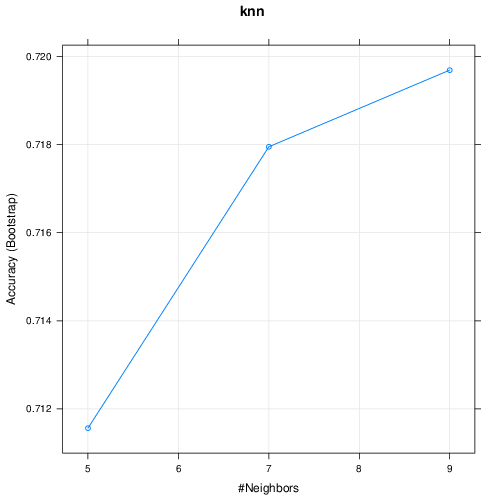
k Nearest Neighbor (knn)

k-Nearest Neighbors 

460 samples
 57 predictor
  2 classes: 'nonspam', 'spam' 

No pre-processing
Resampling: Bootstrapped (25 reps) 
Summary of sample sizes: 460, 460, 460, 460, 460, 460, ... 
Resampling results across tuning parameters:

  k  Accuracy   Kappa    
  5  0.7199522  0.4145264
  7  0.7178108  0.4094426
  9  0.7096166  0.3900999

Accuracy was used to select the optimal model using  the largest value.
The final value used for the model was k = 5.

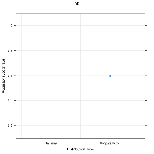
naive Bayse (nb)

Naive Bayes 

460 samples
 57 predictor
  2 classes: 'nonspam', 'spam' 

No pre-processing
Resampling: Bootstrapped (25 reps) 
Summary of sample sizes: 460, 460, 460, 460, 460, 460, ... 
Resampling results across tuning parameters:

  usekernel  Accuracy   Kappa    
  FALSE            NaN        NaN
   TRUE      0.6028973  0.2952961

Tuning parameter 'fL' was held constant at a value of 0
Tuning
 parameter 'adjust' was held constant at a value of 1
Accuracy was used to select the optimal model using  the largest value.
The final values used for the model were fL = 0, usekernel = TRUE and adjust
 = 1.

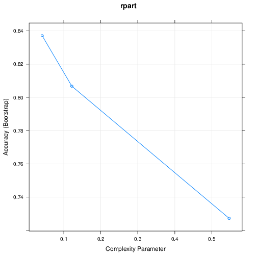
Decision Tree (rpart)

CART 

460 samples
 57 predictor
  2 classes: 'nonspam', 'spam' 

No pre-processing
Resampling: Bootstrapped (25 reps) 
Summary of sample sizes: 460, 460, 460, 460, 460, 460, ... 
Resampling results across tuning parameters:

  cp          Accuracy   Kappa    
  0.04143646  0.8465669  0.6764833
  0.12154696  0.8171015  0.6026779
  0.54696133  0.7282228  0.3510546

Accuracy was used to select the optimal model using  the largest value.
The final value used for the model was cp = 0.04143646.

3層ニューラルネット (nnet)

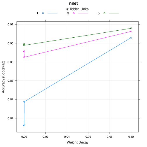
Neural Network 

460 samples
 57 predictor
  2 classes: 'nonspam', 'spam' 

No pre-processing
Resampling: Bootstrapped (25 reps) 
Summary of sample sizes: 460, 460, 460, 460, 460, 460, ... 
Resampling results across tuning parameters:

  size  decay  Accuracy   Kappa    
  1     0e+00  0.8216229  0.6265190
  1     1e-04  0.8649766  0.7150029
  1     1e-01  0.8943997  0.7806125
  3     0e+00  0.8867312  0.7656458
  3     1e-04  0.8924993  0.7754566
  3     1e-01  0.9068637  0.8042872
  5     0e+00  0.8854677  0.7630163
  5     1e-04  0.8927262  0.7746208
  5     1e-01  0.9099463  0.8107649

Accuracy was used to select the optimal model using  the largest value.
The final values used for the model were size = 5 and decay = 0.1.

学習ベクトル量子化ニューラルネットワーク (lvq)

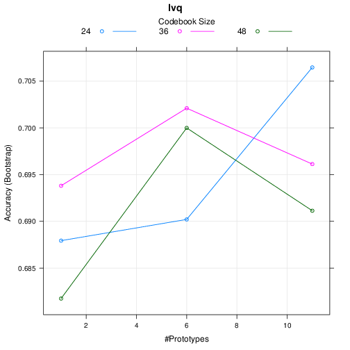
Learning Vector Quantization 

460 samples
 57 predictor
  2 classes: 'nonspam', 'spam' 

No pre-processing
Resampling: Bootstrapped (25 reps) 
Summary of sample sizes: 460, 460, 460, 460, 460, 460, ... 
Resampling results across tuning parameters:

  size  k   Accuracy   Kappa    
  24     1  0.6857730  0.3347985
  24     6  0.7062956  0.3806374
  24    11  0.7030803  0.3728038
  36     1  0.7050989  0.3734752
  36     6  0.7027073  0.3687149
  36    11  0.7073002  0.3852150
  48     1  0.7137609  0.3967521
  48     6  0.7075282  0.3769616
  48    11  0.7139488  0.3970061

Accuracy was used to select the optimal model using  the largest value.
The final values used for the model were size = 48 and k = 11.

Support Vector Machine (svmRadial)

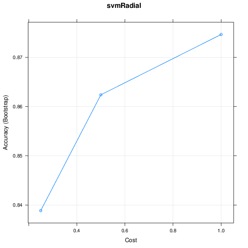
Support Vector Machines with Radial Basis Function Kernel 

460 samples
 57 predictor
  2 classes: 'nonspam', 'spam' 

No pre-processing
Resampling: Bootstrapped (25 reps) 
Summary of sample sizes: 460, 460, 460, 460, 460, 460, ... 
Resampling results across tuning parameters:

  C     Accuracy   Kappa    
  0.25  0.8538915  0.6822898
  0.50  0.8787777  0.7402555
  1.00  0.8877831  0.7611116

Tuning parameter 'sigma' was held constant at a value of 0.02496736
Accuracy was used to select the optimal model using  the largest value.
The final values used for the model were sigma = 0.02496736 and C = 1.

Gradient Boosting Machine (gbm)

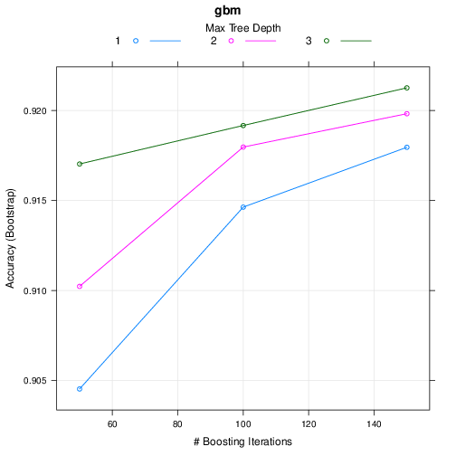
Stochastic Gradient Boosting 

460 samples
 57 predictor
  2 classes: 'nonspam', 'spam' 

No pre-processing
Resampling: Bootstrapped (25 reps) 
Summary of sample sizes: 460, 460, 460, 460, 460, 460, ... 
Resampling results across tuning parameters:

  interaction.depth  n.trees  Accuracy   Kappa    
  1                   50      0.9091337  0.8046674
  1                  100      0.9233847  0.8362842
  1                  150      0.9238490  0.8373352
  2                   50      0.9160698  0.8203036
  2                  100      0.9249554  0.8394724
  2                  150      0.9266512  0.8436142
  3                   50      0.9219410  0.8330738
  3                  100      0.9262219  0.8430003
  3                  150      0.9287916  0.8483900

Tuning parameter 'shrinkage' was held constant at a value of 0.1

Tuning parameter 'n.minobsinnode' was held constant at a value of 10
Accuracy was used to select the optimal model using  the largest value.
The final values used for the model were n.trees = 150, interaction.depth =
 3, shrinkage = 0.1 and n.minobsinnode = 10.

Random Forest (rf)

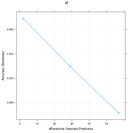
Random Forest 

460 samples
 57 predictor
  2 classes: 'nonspam', 'spam' 

No pre-processing
Resampling: Bootstrapped (25 reps) 
Summary of sample sizes: 460, 460, 460, 460, 460, 460, ... 
Resampling results across tuning parameters:

  mtry  Accuracy   Kappa    
   2    0.9275362  0.8450614
  29    0.9169599  0.8237313
  57    0.9038631  0.7961136

Accuracy was used to select the optimal model using  the largest value.
The final value used for the model was mtry = 2.

Rで判別分析いろいろ（caretパッケージで自動チューニング 8種類）

Background

Summary

方法

結果

結論

感想

References...１つだけ読むなら

Details

使用したデータ

Source code

k Nearest Neighbor (knn)

naive Bayse (nb)

Decision Tree (rpart)

3層ニューラルネット (nnet)

学習ベクトル量子化ニューラルネットワーク (lvq)

Support Vector Machine (svmRadial)

Gradient Boosting Machine (gbm)

Random Forest (rf)

References