※この文章はFeature Selection • mlrを翻訳したものです。一部原文に対して修正した部分、意訳した部分があります。
特徴量選択
データセットが多数の特徴量を含むことは珍しくありません。そのような場合に、多数の特徴量の中から適切な特徴量をいくつか選択することを特徴量選択と呼びます。特徴量選択によってモデルは解釈しやすくなり、学習にかかる時間の短縮や学習器の性能向上も望める場合があります。適切な特徴量を選択する手法はいくつかあり、mlrも複数の手法をサポートしていますが、それらは大きくfilter法とwrapper法と呼ばれるグループに分けられます。
filter法
filter法ではまずそれぞれの特徴量に対して重要度を表す値を計算します。そして、この重要度に応じて特徴量を順位付けし、使う特徴量を選択します。
重要度の計算
重要度はgenerateFilterValuesDate()で計算できます。この関数はいくつかの手法をサポートしています。現在のところ、分類、回帰、生存分析の3種類のタスクがサポートされています。この関数がサポートするすべての手法のリストはIntegrated Filter Methods • mlrで確認できます。
generateFilterValuesDate()を使用する際には、Task()オブジェクトとfilter手法を指定します。
library(mlr)

fv <- generateFilterValuesData(iris.task, "information.gain")
fv
 FilterValues:
 Task: iris-example
           name    type information.gain
 1 Sepal.Length numeric        0.4521286
 2  Sepal.Width numeric        0.2672750
 3 Petal.Length numeric        0.9402853
 4  Petal.Width numeric        0.9554360
ここでfvはFilterValues()オブジェクトであり、fv$dataにデータフレームとして重要度の値が格納されています。フィルター手法はベクトルとして複数指定することもできます。
fv2 <- generateFilterValuesData(iris.task, c("information.gain", "chi.squared"))
fv2
 FilterValues:
 Task: iris-example
           name    type information.gain chi.squared
 1 Sepal.Length numeric        0.4521286   0.6288067
 2  Sepal.Width numeric        0.2672750   0.4922162
 3 Petal.Length numeric        0.9402853   0.9346311
 4  Petal.Width numeric        0.9554360   0.9432359
plotFilterValues()を使えば棒グラフとして重要度を可視化することができます。
plotFilterValues(fv2)
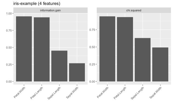
このように、デフォルトでは複数のフィルター手法が指定されていれば手法ごとにプロットが描画されます。
また、現在のところは試験的な段階ですが、plotFilterValuesGGVIS()関数を使うことで、ggvisパッケージを利用したプロットを作成できます。引数はplotFilterValues()と同様です。関数を実行すると、shinyを使用したインタラクティブなグラフが表示され、特徴量のソートや表示する特徴量の数の指定、表示するフィルター手法の切り替えなどの操作ができます(※この関数を利用するためにはGitHubから開発版をインストールする必要があります)。
# devtools::install_github("riebetob/mlr")
# library(mlr)
plotFilterValuesGGVIS(fv2)
話を戻しますが、今回利用した重要度の指標であるinformation.gainによればPetalWidthとPetal.Lengthが目的変数Speciesに対して多くの情報量を持っている特徴量だということになります。
フィルター法による特徴量の選択
重要度を計算したら、次はそれを実際にタスクに反映したくなりますね。filterFeatures()関数を使うと、重要度が低かった特徴量を除外した新しいタスクオブジェクトを作成できます。
ここで課題になるのは、重要度に基づいて特徴量をどのように選択するのか、という点です。これにはいくつかの方法があります。
-
abs残す特徴量の絶対数を決めておいて、重要度の上位からその個数だけ特徴量を選択する。 -
perc残す特徴量の割合を決めておいて、重要度の上位からその割合になるまで特徴量を選択する。 -
threshold重要度のしきい値を決めておいて、重要度がしきい値が上回った特徴量はすべて残す。
これから示すように、filterFeatures()はこれら3つの手法をサポートしています。それだけでなく、判断に用いる重要度の計算手法をここで指定してあらためて計算することもできます。もし他で先に計算した重要度を使いたければ、fval=に指定します。
# 上位2つの特徴量を残す場合(& 重要度もここで同時に計算する場合)
filtered.task <- filterFeatures(iris.task, method = "information.gain", abs = 2)

# 上位25%の特徴量を残す場合(& 重要度は過去に計算したものを使う場合)
filtered.task <- filterFeatures(iris.task, fval = fv, perc = .25)

# しきい値を0.5としてこれを上回る重要度の特徴量をすべて残す場合
filtered.task <- filterFeatures(iris.task, fval = fv, threshold = .5)

filtered.task
 Supervised task: iris-example
 Type: classif
 Target: Species
 Observations: 150
 Features:
    numerics     factors     ordered functionals
           2           0           0           0
 Missings: FALSE
 Has weights: FALSE
 Has blocking: FALSE
 Has coordinates: FALSE
 Classes: 3
     setosa versicolor  virginica
         50         50         50
 Positive class: NA
学習器とフィルター法を融合する
フィルター法による特徴量選択の結果はテストデータによって異なる可能性があります。したがって、適切に試験を行うのであれば、例えばクロスバリデーションの繰り返しの都度、特徴量選択をしたほうが望ましいといえます。
学習器はmakeFilterWrapper()関数を使うことでフィルター手法と融合させることができます。この関数を適用すると、学習器は新たなクラス属性FilterWrapper()を付与され、クロスバリデーションなどの性能評価のステップごとに特徴量選択が行われるようになります。
次に示す例では、irisを対象に特徴量選択を行ってk-最近傍法を適用します。そして、性能は10分割クロスバリデーションでmmceを計算して評価します。特徴量選択のステップでは、重要度としてinformation.gainを使用し、2つの特徴量を選択します。
lrn <- makeFilterWrapper(learner = "classif.fnn", fw.method = "information.gain", fw.abs = 2)
rdesc <- makeResampleDesc("CV", iters = 10)
r <- resample(learner = lrn, task = iris.task, resampling = rdesc, show.info = FALSE, models = TRUE)
r$aggr
 mmce.test.mean
     0.03333333
ところで、結局どの特徴量が使われたのか気になりますね。幸いなことに、今resample()を呼び出した際にmodels = TRUEを指定していました。これにより、r$modelsに個々の繰り返しで得られたモデルがリストで格納されます。どの特徴量が使われたのか知るためには、それぞれのモデルにgetFilterdFeatures()関数を適用します。
sfeats <- sapply(r$models, getFilteredFeatures)
table(sfeats)
 sfeats
 Petal.Length  Petal.Width
           10           10
今回の例では特徴量選択の結果は非常に安定していました。Sepal.LengthとSepal.Widthは一度も選ばれることがありませんでした。
選択する特徴量の数に対するチューニング
これまで示した例では特徴量の個数や割合を任意に決めていました。しかし、特徴量の数が性能に関わってくるのであれば、学習器の性能に対して最適な特徴量の数をチューニングによって決めたいところです。
mlrでは、percのような特徴量選択に関わるパラメータも簡単にチューニングの対象にできます。
次に示す例ではBostonHousingデータセットを対象にした回帰問題を扱います。モデルとしては線形回帰モデルを使用し、特徴量の数の割合に対してチューニングを行います。性能は3分割クロスバリデーションによりmseを計算して評価します。パラメータ探索の手法はグリッドサーチを用います。
lrn <- makeFilterWrapper(learner = "regr.lm", fw.method = "chi.squared")
ps <- makeParamSet(makeDiscreteParam("fw.perc", values = seq(0.2, 0.5, 0.05)))
rdesc <- makeResampleDesc("CV", iters = 3)
res <- tuneParams(lrn, task = bh.task, resampling = rdesc, par.set = ps, control = makeTuneControlGrid())
 [Tune] Started tuning learner regr.lm.filtered for parameter set:

             Type len Def                         Constr Req Tunable Trafo
 fw.perc discrete   -   - 0.2,0.25,0.3,0.35,0.4,0.45,0.5   -    TRUE     -

 With control class: TuneControlGrid

 Imputation value: Inf

 [Tune-x] 1: fw.perc=0.2
 [Tune-y] 1: mse.test.mean=35.4849486; time: 0.0 min

 [Tune-x] 2: fw.perc=0.25
 [Tune-y] 2: mse.test.mean=35.4849486; time: 0.0 min

 [Tune-x] 3: fw.perc=0.3
 [Tune-y] 3: mse.test.mean=35.4717346; time: 0.0 min

 [Tune-x] 4: fw.perc=0.35
 [Tune-y] 4: mse.test.mean=31.4755980; time: 0.0 min

 [Tune-x] 5: fw.perc=0.4
 [Tune-y] 5: mse.test.mean=31.4755980; time: 0.0 min

 [Tune-x] 6: fw.perc=0.45
 [Tune-y] 6: mse.test.mean=31.4873377; time: 0.0 min

 [Tune-x] 7: fw.perc=0.5
 [Tune-y] 7: mse.test.mean=31.4873377; time: 0.0 min

 [Tune] Result: fw.perc=0.4 : mse.test.mean=31.4755980
チューニングの間に探索されたfw.percの値はres$pot.pathを通じて確認できます。
as.data.frame(res$opt.path)
   fw.perc mse.test.mean dob eol error.message exec.time
 1     0.2      35.48495   1  NA          <NA>     0.232
 2    0.25      35.48495   2  NA          <NA>     0.188
 3     0.3      35.47173   3  NA          <NA>     0.194
 4    0.35      31.47560   4  NA          <NA>     0.169
 5     0.4      31.47560   5  NA          <NA>     0.168
 6    0.45      31.48734   6  NA          <NA>     0.167
 7     0.5      31.48734   7  NA          <NA>     0.158
チューニングの結果得られた最適値は次のように確認します。
res$x
 $fw.perc
 [1] 0.4
res$y
 mse.test.mean
       31.4756
したがって、チューニング結果のパラメータを用いて新しく学習器を作成したければ次のようにします。
lrn <- makeFilterWrapper(learner = "regr.lm", fw.method = "chi.squared", fw.perc = res$x$fw.perc)
mod <- train(lrn, bh.task)
mod
 Model for learner.id=regr.lm.filtered; learner.class=FilterWrapper
 Trained on: task.id = BostonHousing-example; obs = 506; features = 13
 Hyperparameters: fw.method=chi.squared,fw.perc=0.4
今回選択された特徴量は次のとおりです。
getFilteredFeatures(mod)
[1] "crim" "zn" "dis" "rad" "lstat"
他の例として、複数の性能指標を用いたチューニング(multi-criteria tuning)の例を示します。今回はSonarデータセットを対象に、chi.squaredを重要度の指標とした特徴量選択を行った後に線形判別分析を行います。そして、チューニング対象は重要度選択のしきい値とします。チューニングにあたっては、偽陽性率(fpr)および偽陽性率(fnr)の2つの性能指標を最小化するように探索を行います。探索方法にはランダムサーチを用います。
lrn <- makeFilterWrapper(learner = "classif.lda", fw.method = "chi.squared")
ps <- makeParamSet(makeNumericParam("fw.threshold", lower = 0.1, upper = 0.9))
rdesc <- makeResampleDesc("CV", iters = 10)
res <- tuneParamsMultiCrit(lrn, task = sonar.task, resampling = rdesc, par.set = ps,
                           measures = list(fpr, fnr), control = makeTuneMultiCritControlRandom(maxit = 50L),
                           show.info = FALSE)
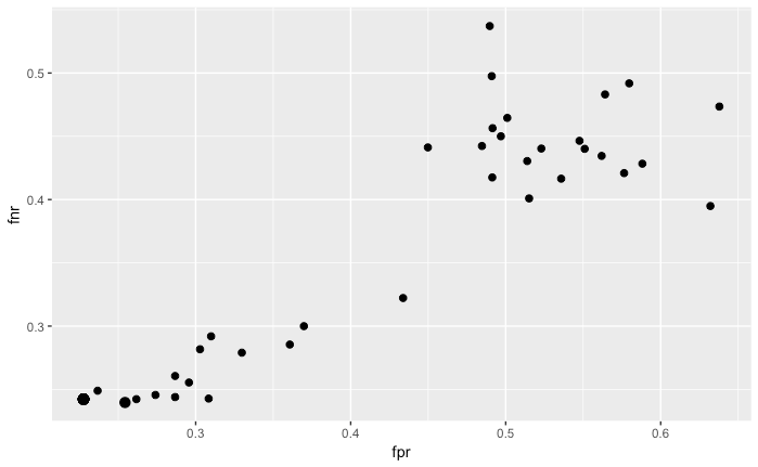
チューニング結果はplotTuneMultiCritResult()関数を使うと可視化できます。プロットはfprとfnrを軸とした散布図として描かれ、パレートフロントに対応する点が少し大きなポイントサイズで示されます。
plotTuneMultiCritResult(res)
wrapper法
wrapper法は実際の学習器の性能を基準にして特徴量を選択する手法です。つまり、特徴量を選択するためには、異なる特徴量の組み合わせに対して学習と評価を何度も繰り返す必要があります。
wrapper法を使うためには次の点を決める必要があります。
- 性能の評価手法。これには特徴量を選択するための基準となる性能指標の選択と、リサンプリング手法の選択の両方が含まれる。
- どの学習手法を使うか。
- 特徴量の可能な組み合わせのうち、どれだけの範囲を探索するのか。
探索方法を定義する関数は、makeFeatSelControl<探索手法>のような名前になっています。次の手法が利用可能です。
- 網羅的(Exhaustive)探索:
makeFeatSelControlExhaustive() - 遺伝的アルゴリズム:
makeFeatSelControlGA() - ランダムサーチ:
makeFeatSelControlRandom() - シーケンシャルサーチ:
makeFeatSelControlSequential()
wrapper法による特徴量の選択
特徴量選択はselectFeatures()関数で実行します。
次に示す例ではcancerデータ(Wisconsin Prognostic Breast Cancer: TH.data::wpbc())を対象に、ランダムサーチを行います。学習手法はコックス比例ハザードモデルを用います。性能はホールドアウト法で計算したc-index(concordance index)により評価します。
# 探索方法の定義
ctrl <- makeFeatSelControlRandom(maxit = 20L)
ctrl
 FeatSel control: FeatSelControlRandom
 Same resampling instance: TRUE
 Imputation value: <worst>
 Max. features: <not used>
 Max. iterations: 20
 Tune threshold: FALSE
 Further arguments: prob=0.5
ctrlはFeatSelControl()オブジェクトであり、探索方法とパラメータに関する情報を含んでいます。
rdesc <- makeResampleDesc("Holdout")
sfeats <- selectFeatures(learner = "surv.coxph", task = wpbc.task, resampling = rdesc,
                         control = ctrl, show.info = FALSE)
sfeats
 FeatSel result:
 Features (20): mean_radius, mean_perimeter, mean_area, mean_smoothness, mean_concavity, mean_concavepoints, mean_fractaldim, SE_radius, SE_area, SE_smoothness, SE_compactness, SE_concavepoints, SE_fractaldim, worst_radius, worst_perimeter, worst_area, worst_compactness, worst_concavity, worst_fractaldim, tsize
 cindex.test.mean=0.6604867
sfeatsはFeatSelResult()オブジェクトです。選択された特徴量と、その特徴量を用いた場合の性能指標は次のように参照できます。
sfeats$x
  [1] "mean_radius"        "mean_perimeter"     "mean_area"
  [4] "mean_smoothness"    "mean_concavity"     "mean_concavepoints"
  [7] "mean_fractaldim"    "SE_radius"          "SE_area"
 [10] "SE_smoothness"      "SE_compactness"     "SE_concavepoints"
 [13] "SE_fractaldim"      "worst_radius"       "worst_perimeter"
 [16] "worst_area"         "worst_compactness"  "worst_concavity"
 [19] "worst_fractaldim"   "tsize"
sfeats$y
 cindex.test.mean
        0.6604867
次に示す例では、BostonHousingに線形回帰を適用します。特徴量の探索にはシーケンシャルサーチを用い、最適化する性能指標にはmseを用います。method = "sfs"(シーケンシャルフォワードサーチ)を指定すると、特徴量0個から開始して性能指標が改善しなくなるまで特徴量を加えるような探索が行われます。これ以外のシーケンシャルサーチの手法については、?FeatSelControlのヘルプ内のmakeFeatSelControlSequentialの部分を確認してください。また、例ではalpha = 0.02を指定していますが、これは性能指標の改善幅が0.02を下回ったら探索をやめるという指定です。
ctrl <- makeFeatSelControlSequential(method = "sfs", alpha = 0.02)

rdesc <- makeResampleDesc("CV", iters = 10)
sfeats <- selectFeatures(learner = "regr.lm", task = bh.task, resampling = rdesc, control = ctrl,
                         show.info = FALSE)
sfeats
 FeatSel result:
 Features (11): crim, zn, chas, nox, rm, dis, rad, tax, ptratio, b, lstat
 mse.test.mean=23.7885926
analyzeFeatSelResult()関数を用いると、特徴量選択の過程を確認できます。
analyzeFeatSelResult(sfeats)
 Features         : 11
 Performance      : mse.test.mean=23.7885926
 crim, zn, chas, nox, rm, dis, rad, tax, ptratio, b, lstat

 Path to optimum:
 - Features:    0  Init   :                       Perf = 84.58  Diff: NA  *
 - Features:    1  Add    : lstat                 Perf = 38.802  Diff: 45.779  *
 - Features:    2  Add    : rm                    Perf = 31.426  Diff: 7.3758  *
 - Features:    3  Add    : ptratio               Perf = 28.089  Diff: 3.3372  *
 - Features:    4  Add    : dis                   Perf = 27.219  Diff: 0.86968  *
 - Features:    5  Add    : nox                   Perf = 25.925  Diff: 1.2936  *
 - Features:    6  Add    : b                     Perf = 25.318  Diff: 0.60727  *
 - Features:    7  Add    : zn                    Perf = 24.97  Diff: 0.34802  *
 - Features:    8  Add    : chas                  Perf = 24.681  Diff: 0.28861  *
 - Features:    9  Add    : crim                  Perf = 24.653  Diff: 0.028028  *
 - Features:   10  Add    : rad                   Perf = 24.32  Diff: 0.33391  *
 - Features:   11  Add    : tax                   Perf = 23.789  Diff: 0.53094  *

 Stopped, because no improving feature was found.
学習器との融合
makeFeatSelWrapper()関数を用いることで、特徴量選択の手法と学習器を組み合わせることができます。特徴量選択の手法の中には探索方法、最適化の対象とする学習器の性能指標、性能評価のためのリサンプリング手法の指定が含まれています。訓練の間、特徴量は指定した方法で選択されます。すなわち、学習器の訓練は選択された特徴量を用いて実行されます。
rdesc <- makeResampleDesc("CV", iters = 3)
lrn <- makeFeatSelWrapper("surv.coxph", resampling = rdesc,
                          control = makeFeatSelControlRandom(maxit = 10), show.info = FALSE)
mod <- train(lrn, task = wpbc.task)
mod
 Model for learner.id=surv.coxph.featsel; learner.class=FeatSelWrapper
 Trained on: task.id = wpbc-example; obs = 194; features = 32
 Hyperparameters:
特徴量選択の結果はgetFeatSelResult()で確認できます。
sfeats <- getFeatSelResult(mod)
sfeats
 FeatSel result:
 Features (9): mean_texture, mean_area, SE_perimeter, SE_area, SE_smoothness, SE_fractaldim, worst_radius, worst_smoothness, pnodes
 cindex.test.mean=0.6502295
今回、次の特徴量が選択されました。
sfeats$x
 [1] "mean_texture"     "mean_area"        "SE_perimeter"
 [4] "SE_area"          "SE_smoothness"    "SE_fractaldim"
 [7] "worst_radius"     "worst_smoothness" "pnodes"
今度はさきほど定義した学習器の性能を5分割クロスバリデーションで確認してみましょう。つまり、5回の繰り返しそれぞれで、指定した方法による特徴量の選択が行われます。
out.rdesc = makeResampleDesc("CV", iters = 5)

r = resample(learner = lrn, task = wpbc.task, resampling = out.rdesc, models = TRUE,
             show.info = FALSE)
r$aggr
 cindex.test.mean
         0.598899
各繰り返しで採用された特徴量のセットは次のように確認できます。
lapply(r$models, getFeatSelResult)
 [[1]]
 FeatSel result:
 Features (17): mean_radius, mean_texture, mean_perimeter, mean_smoothness, mean_concavity, mean_concavepoints, mean_symmetry, mean_fractaldim, SE_perimeter, SE_compactness, SE_concavity, SE_fractaldim, worst_texture, worst_smoothness, worst_concavity, worst_concavepoints, pnodes
 cindex.test.mean=0.6437948

 [[2]]
 FeatSel result:
 Features (19): mean_radius, mean_texture, mean_perimeter, mean_area, mean_smoothness, mean_compactness, mean_concavity, mean_symmetry, mean_fractaldim, SE_radius, SE_smoothness, SE_concavepoints, SE_symmetry, SE_fractaldim, worst_texture, worst_smoothness, worst_concavity, worst_symmetry, worst_fractaldim
 cindex.test.mean=0.7219501

 [[3]]
 FeatSel result:
 Features (13): mean_radius, mean_perimeter, mean_smoothness, mean_fractaldim, SE_radius, SE_area, SE_smoothness, SE_fractaldim, worst_radius, worst_texture, worst_perimeter, worst_area, worst_compactness
 cindex.test.mean=0.5942115

 [[4]]
 FeatSel result:
 Features (12): mean_radius, mean_perimeter, mean_compactness, mean_concavepoints, mean_fractaldim, SE_perimeter, SE_smoothness, SE_concavepoints, worst_texture, worst_smoothness, worst_symmetry, pnodes
 cindex.test.mean=0.6771394

 [[5]]
 FeatSel result:
 Features (17): mean_compactness, mean_concavity, mean_symmetry, mean_fractaldim, SE_radius, SE_perimeter, SE_area, SE_concavity, SE_concavepoints, SE_fractaldim, worst_radius, worst_texture, worst_smoothness, worst_compactness, worst_concavepoints, worst_symmetry, tsize
 cindex.test.mean=0.5974155