RとRcppで緯度経度から都道府県と行政区域を高速に検索(したかった)

前回(Rで緯度経度から都道府県を求める - Qiita)のやり方でも行政区域まで10ms程度で検索できるが、たくさん検索したかったのでRcppで高速化を試みた。結果は

前回のやり方の概要

行政区域のセントロイドと目標座標の間の距離を求めておいて、最も距離の短かった行政区域の情報を参照する。

library(sf)

# 日本地図のシェープファイルを読み込む
f <- "data_source/N03-160101_GML/N03-16_160101.shp"
japan <- st_read(f)

jpn_cent <- st_centroid(japan) # セントロイド計算
cent_mat <- t(matrix(unlist(jpn_cent$geometry), nrow=2)) # 地点をmatrixに

find_admin_old <- function(point){ # 最寄りの行政区域の情報を抽出
  jpn_cent[which.min(sqrt(rowSums(t(t(cent_mat) - point)^2))),]
}
find_pref_old <- function(point){  # 都道府県名のみ抽出
  as.character(find_admin_old(point)$N03_001)
}

> p1 <- c(138.5, 37.1) # 新潟県
> find_admin_old(p1)
Simple feature collection with 1 feature and 5 fields
geometry type:  POINT
dimension:      XY
bbox:           xmin: 138.3375 ymin: 37.12011 xmax: 138.3375 ymax: 37.12011
epsg (SRID):    NA
proj4string:    +proj=longlat +ellps=GRS80 +no_defs
      N03_001 N03_002 N03_003 N03_004 N03_007                       geometry
40776  新潟県    <NA>    <NA>  上越市   15222 POINT(138.337517708344 37.1...

これで10万件調べると15分くらいかかる。

Rcpp

おそらくwhich.min(sqrt(rowSums(t(t(cent_mat) - point)^2)))の部分が遅かろうと思われるので、ここだけRcppで置き換えた。

find_near_point.cpp

# include <Rcpp.h>
using namespace Rcpp;

// [[Rcpp::export]]
NumericVector find_near_point(NumericVector lat, NumericVector lng,
                              NumericVector p1,  NumericVector p2) {
  NumericVector result (p1.length());
  for(int i=0; i<p1.length(); ++i){
    NumericVector dist (lat.length());
    for(int j=0; j<lat.length(); ++j){
      dist[j] = pow(lat[j] - p1[i], 2.0) + pow(lng[j] - p2[i], 2.0);
    }
    result[i] = std::min_element(dist.begin(), dist.end()) - dist.begin() + 1;
  }
  return result;
}

ちなみに距離を計算するところ、ベクトルとスカラーの演算としてまとめてやったら早くなるかと思ったら逆に遅くなった。「R言語徹底解説」をふわっと読んだ感じだとベクトルの演算っぽく書けるのはただの糖衣構文らしい。

ファイルを支度したらRからコンパイルして使う。また、引数の与え方が変わってしまったのでセントロイドの緯度経度情報をベクトルにしておく。

lat <- cent_mat[,2]
lng <- cent_mat[,1]

library(Rcpp)
sourceCpp("find_near_point.cpp")

find_admin <- function(plat, plng){ # 最寄りの行政区域
  #jpn_cent[which.min(sqrt(rowSums(t(t(cent_mat) - point)^2))),]
  jpn_cent[find_near_point(lat, lng, plat, plng),]
}
find_pref <- function(plat, plng){  # 都道府県名のみ抽出
  as.character(find_admin(plat, plng)$N03_001)
}

結果

10万件3分くらい。4〜5倍早くなった感じ。

test_lng <- runif(100000, 130, 145)
test_lat <- runif(100000, 30, 45)
test_mat <- matrix(c(test_lng, test_lat), ncol=2)

system.time(find_pref(test_lat, test_lng))
system.time(apply(test_mat, 1, find_pref_old))

> system.time(find_pref(test_lat, test_lng))
   ユーザ   システム       経過  
   131.206     43.474    190.491 
> system.time(apply(test_mat, 1, find_pref_old))
   ユーザ   システム       経過  
   532.952    335.576    882.854 

もうちょい早くしたいところ。

追記

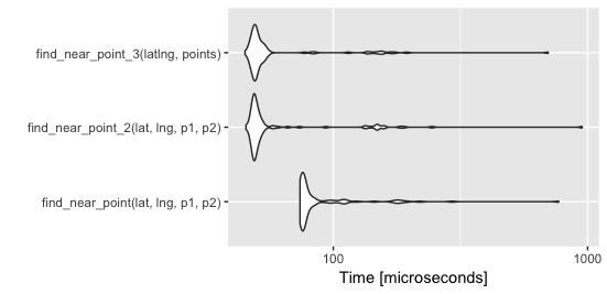
25%減(当社比)。関数呼び出しのオーバーヘッドを減らすように注意すれば多少早くなる。ついでにmatrix対応版を作った。速度には関係ないみたい。あとmicrobenchmarkの存在を知った。便利。

# include <Rcpp.h>
using namespace Rcpp;

// [[Rcpp::export]]
NumericVector find_near_point(NumericVector lat, NumericVector lng,
                              NumericVector p1,  NumericVector p2) {
  NumericVector result (p1.length());
  for(int i=0; i<p1.size(); ++i){
    NumericVector dist (lat.size());
    for(int j=0; j<lat.size(); ++j){
      dist[j] = pow(lat[j] - p1[i], 2.0) + pow(lng[j] - p2[i], 2.0);
    }
    result[i] = std::min_element(dist.begin(), dist.end()) - dist.begin() + 1;
  }
  return result;
}

// [[Rcpp::export]]
NumericVector find_near_point_2(NumericVector lat, NumericVector lng,
                                NumericVector p1,  NumericVector p2) {
  NumericVector result (p1.length());
  int p1s = p1.size();
  int lats = lat.size();
  for(int i=0; i<p1s; ++i){
    NumericVector dist (lats);
    for(int j=0; j<lats; ++j){
      dist[j] = pow(lat[j] - p1[i], 2.0) + pow(lng[j] - p2[i], 2.0);
    }
    result[i] = std::min_element(dist.begin(), dist.end()) - dist.begin() + 1;
  }
  return result;
}

// [[Rcpp::export]]
NumericVector find_near_point_3(NumericMatrix latlng, 
                                NumericMatrix points) {
  int p_nrow = points.nrow();
  int l_nrow = latlng.nrow();
  NumericVector result (p_nrow);
  for(int i=0; i < p_nrow; ++i){
    NumericVector dist (l_nrow);
    for(int j=0; j < l_nrow; ++j){
      dist[j] = pow(latlng(j, 0) - points(i, 0), 2.0) +
                pow(latlng(j, 1) - points(i, 1), 2.0);
    }
    result[i] = std::min_element(dist.begin(), dist.end()) - dist.begin() + 1;
  }
  return result;
}

/*** R
library(microbenchmark)
lat = runif(100)
lng = runif(100)
latlng = matrix(c(lat, lng), ncol = 2)
p1 = runif(100)
p2 = runif(100)
points = matrix(c(p1, p2), ncol = 2)

result <- microbenchmark(
  find_near_point(lat,lng,p1,p2),
  find_near_point_2(lat,lng,p1,p2),
  find_near_point_3(latlng, points)
  )
ggplot2::autoplot(result)
result
*/