PennylaneでQAOA

Pennylaneでの実装

Pennylane公式のQAOAのチュートリアルがちょっとだけ使いづらいので、簡単にしました。
qaoaクラスを使って楽をします。
なぜか公式チュートリアルだと、「最後の最適化は自分で頑張ってね」で終わっています、、
以下は最適化も含むコードです。

import pennylane as qml
import numpy as np
import random
from pennylane import qaoa
from networkx import Graph

# Defines the wires and the graph on which MaxCut is being performed
n_qubits = 3
n_layers = 2
wires = range(n_qubits)
edges = [(0, 1), (1, 2), (2, 0)]
graph = Graph(edges)

# Defines the QAOA cost and mixer Hamiltonians
cost_h, mixer_h = qaoa.maxcut(graph)
# Defines a layer of the QAOA ansatz from the cost and mixer Hamiltonians
def qaoa_layer(gamma, alpha):
    qaoa.cost_layer(gamma, cost_h)
    qaoa.mixer_layer(alpha, mixer_h)
dev = qml.device('lightning.qubit', wires=len(wires))
# Repeatedly applies layers of the QAOA ansatz
def circuit(var, **kwargs):
    var_2d_array = np.reshape(var,(2,n_layers))
    for w in wires:
        qml.Hadamard(wires=w)

    qml.layer(qaoa_layer, n_layers, var_2d_array[0], var_2d_array[1])

# Defines the QAOA cost function
cost = qml.ExpvalCost(circuit, cost_h, dev)
from scipy.optimize import minimize
import time

var_init = np.random.uniform(low=-1, high=1, size=(2*n_layers)) # one-dimensional array
hist_cost = []
var = var_init

count = 0
def cbf(Xi):
    global count
    global hist_cost
    count += 1
    cost_now = cost(Xi)
    hist_cost.append(cost_now)
    print('iter = '+str(count)+' | cost = '+str(cost_now))


t1 = time.time()
result = minimize(fun=cost, x0=var_init, method='Nelder-Mead', callback=cbf, options={"maxiter":50})

t2 = time.time() 
elapsed_time = t2-t1
print(f"Time：{elapsed_time}")
print(f"Time per iteration : {elapsed_time/50}")       
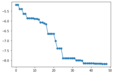
from matplotlib import pyplot as plt
plt.plot(hist_cost,'o-') 

iter = 1 | cost = -3.790512266733385
iter = 2 | cost = -3.9674137541481724
iter = 3 | cost = -3.997367263730413
iter = 4 | cost = -3.999999974706611
Time：13.195805311203003
Time per iteration : 0.26391610622406003

・遅いです。Blueqatのほうが圧倒的に早いです。