PennyLaneのβ版機能: Tensor network simulation

最近、量子ゲートのシミュレーション手法として話題のTensor network simulation。
PennyLaneでも使えたらいいなと思っていました。
β版機能として一応存在しています。

qml.beta
This module contains experimental, contributed, and beta functions and features.

pennylane.beta.devices Package
This package contains experimental plugin devices for PennyLane.

動作保証は何も有りませんよ、ということになっています。
結論から言うと、どうもうまく動かないようです。

追記
申告したところ、やはりバグだということでした。
default.tensor does not return correlated samples #1419
https://github.com/PennyLaneAI/pennylane/issues/1419

やってみる

が、とりあえずやってみます。

Tensornetworkのv03が必要です。
#pip install tensornetwork==0.3
Pennylaneのversionは0.15.0を使用します。

import pennylane as qml
from pennylane import numpy as np

回路出力集計用の関数です。

def sample_to_counts(sample):
    n_qubits, n_shots = np.shape(sample)
    sample_bin = (1+sample)/2
    weights = [2**i for i in range(n_qubits)]
    sample_dec = np.average(sample_bin,axis=0,weights=weights)*np.sum(weights) # sum b_n*2^n
    sample_dec = sample_dec.astype('int8')
    u, freq = np.unique(sample_dec, return_counts=True) # count frequency
    counts=dict()
    for i,j in zip(u,freq):
        counts.setdefault(format(i, '0'+str(n_qubits)+'b'),j)
    for i in range (2**n_qubits):
        counts.setdefault(format(i, '0'+str(n_qubits)+'b'),0) # zero-padding
    return counts

3 qubit のGHZ状態を作ります。|000>+|111>です。
まずはテンソルネットワークではない、通常の状態ベクトル計算です。

n_qubits = 3
#dev = qml.device("default.tensor", wires=n_qubits, shots=100, representation="mps")
dev = qml.device("default.qubit", wires=n_qubits, shots=100)

@qml.qnode(dev)
def circuit():
    qml.Hadamard(wires=[0])
    for i in range(0,n_qubits-1):
        qml.CNOT(wires=[i,i+1])
    return [qml.sample(qml.PauliZ(i)) for i in range(n_qubits)]

回路図は、¹

print(circuit.draw())

0: ──H──╭C──────┤ Sample[Z]
1: ─────╰X──╭C──┤ Sample[Z]
2: ─────────╰X──┤ Sample[Z]

結果を取ります。

counts = sample_to_counts(circuit())

import matplotlib.pyplot as plt
plt.bar(counts.keys(), counts.values());
plt.xlabel('bitstrings');
plt.ylabel('counts');
plt.xticks(rotation=90);
#print(circuit.draw())

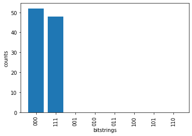
ちゃんとGHZ状態になっています。

次にテンソルネットワークシミュレーションをやります。

deviceを default.tensor にすればよいです。
特に、厳密法と近似(MPS)が選べます。ひとまず厳密で。

n_qubits = 3
dev = qml.device("default.tensor", wires=n_qubits, shots=100, representation="exact")
#dev = qml.device("default.qubit", wires=n_qubits, shots=100)

@qml.qnode(dev)
def circuit():
    qml.Hadamard(wires=[0])
    for i in range(0,n_qubits-1):
        qml.CNOT(wires=[i,i+1])
    return [qml.sample(qml.PauliZ(i)) for i in range(n_qubits)]

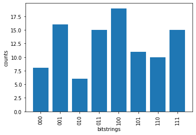
なぜか全然違う状態が出てきています。
ちょっと意味不明です。

計算時間

計算時間も比較してみます。Tensor network のほうが速いはずなのですが・・・
15 qubit GHZにおいて
state vector : 0.014 s
tensor network (exact) : 0.10 s
tensor network (mps) : 0.12 s
となり、テンソルネットワークのほうが遅いという結果になりました。

ただ、これはテンソルネットワークへの置き換えと状態計算を両方含んだ計算時間になっています。

まとめ

PennylaneのTensor network simulationは事実上未実装？
出力がおかしい感じです。
Communityにあげようと思います。

もしqiskitのmpl形式できれいな回路図を出したい場合は以下のようにします。pennylane-qiskitをpipした跡に、dev = qml.device("qiskit.aer", wires=n_qubits)のようにしてqiskitバックエンドをデバイスに設定します。次に回路を一度実行します。たとえばmy_circuit(params)。その後立て続けにdev._circuit.draw('mpl')を実行します。すると、最後に実行された回路(my_circuit)の回路図がmplで出てきます。 ↩

PennyLaneのβ版機能を試してみる(Tensor network simulation)

PennyLaneのβ版機能: Tensor network simulation

やってみる

計算時間

まとめ