はじめに

「tf.kerasでFReLUを実装」の記事を書かれている方がいらっしゃったので、それを使ってみようと思います。
https://qiita.com/rabbitcaptain/items/26304b5a5e401db5bae2

MNISTの判定をやってみる

FReLU()とそれから呼ばれるmax_unit()は上記の記事のをそのまま使います。（もし試す場合は最初に実行してください）
Functionalモデルで実装されてるようなので、Functionalモデルで作成します。

from tensorflow.keras.layers import Input, Activation
from tensorflow.keras.models import Model
from tensorflow.keras.layers import Conv2D, MaxPooling2D, GlobalAveragePooling2D
from tensorflow.keras.layers import Dense, Dropout, BatchNormalization
from tensorflow.keras.optimizers import Adam

def createModel():
  main_input = Input(shape=(28,28,1,), name='main_input')
  x = Conv2D(32, kernel_size=(3, 3), padding='same')(main_input)
  x = FReLU(x)
  x = Conv2D(32, kernel_size=(3, 3), padding='same')(x)
  x = FReLU(x)

  x = MaxPooling2D()(x)

  x = Conv2D(32, kernel_size=(3, 3), padding='same')(x)
  x = FReLU(x)
  x = Conv2D(32, kernel_size=(3, 3), padding='same')(x)
  x = FReLU(x)

  x = MaxPooling2D()(x)

  x = Conv2D(32, kernel_size=(3, 3), padding='same')(x)
  x = FReLU(x)
  x = Conv2D(32, kernel_size=(3, 3), padding='same')(x)
  x = FReLU(x)

  x = GlobalAveragePooling2D()(x)
  x = Dense(units=10, activation='softmax')(x)

  return Model(inputs=[main_input], outputs=[x])

MNISTのデータをロードして加工します。

import tensorflow.keras as keras
mnist = keras.datasets.mnist

(train_images, train_labels), (test_images, test_labels) = mnist.load_data()

import numpy as np
train_images_norm = (train_images / 255.0).astype(np.float16)
test_images_norm = (test_images / 255.0).astype(np.float16)

train_images_norm_rs = train_images_norm.reshape(-1, 28, 28, 1)
test_images_norm_rs  = test_images_norm.reshape(-1, 28, 28, 1)

train_labels_ct = keras.utils.to_categorical(train_labels, 10)
test_labels_ct = keras.utils.to_categorical(test_labels, 10)

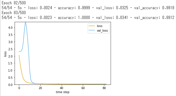
今回も「Ｒａｓｐｂｅｒｒｙ　Ｐｉではじめる機械学習　基礎からディープラーニングまで」に載っていた学習結果の表示用関数を使います。

import matplotlib.pyplot as plt
def plotHistory(history):
    # 損失関数のグラフの軸ラベルを設定
    plt.xlabel('time step')
    plt.ylabel('loss')
    # グラフ縦軸の範囲を0以上と定める
    plt.ylim(0, max(np.r_[history.history['val_loss'], history.history['loss']]))
    # 損失関数の時間変化を描画
    val_loss, = plt.plot(history.history['val_loss'], c='#56B4E9')
    loss, = plt.plot(history.history['loss'], c='#E69F00')
    # グラフの凡例（はんれい）を追加
    plt.legend([loss, val_loss], ['loss', 'val_loss'])
    # 描画したグラフを表示
    plt.show()

モデルの作成及びコンパイル後、学習を実行します。

from tensorflow.keras.callbacks import EarlyStopping

model = createModel()
# モデルのコンパイル
model.compile(loss='categorical_crossentropy', optimizer=Adam(lr=0.0001), metrics=['accuracy'])
model.summary()
# モデルの学習
early_stopping = EarlyStopping(monitor='val_loss', mode='min', patience=30)

plotHistory(
  model.fit(
    train_images_norm_rs
    ,train_labels_ct
    ,epochs=500
    ,validation_split=0.1
    ,batch_size=1000
    ,verbose=2
    ,callbacks=[early_stopping]
  ) 
)

判定を行ってみます。

result_pred = model.predict(test_images_norm_rs, verbose=0)

result = np.argmax(result_pred, axis=1)

print('ターゲット')
print(test_labels)
print('ディープラーニングによる予測')
print(result)

# データ数をtotalに格納
total = len(test_images_norm_rs)
# ターゲット（正解）と予測が一致した数をsuccessに格納
success = sum(result==test_labels)

# 正解率をパーセント表示
print('正解率')
print(100.0*success/total)

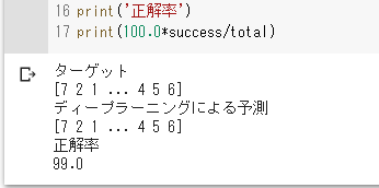
結果

適当に作ったモデルでしたが、99%の正解率となりました。

KerasでFReLUを使ってみる

はじめに

MNISTの判定をやってみる

結果