shifting factorは画像生成モデルや動画生成モデルにおいてSampling,Trainingのtime-step tを歪ませることでDiTの学習を高速化(効率化)や生成品質を向上する事を目標に設定されている。これについて自分なりに調べてみる。
linear-quadratic(Movie Gen)
MetaのMovie Genではlinear-quadraticという前半(25step)で一次関数、後半(25step)で二次関数となるスケジュールである。

ここで前半の一次関数(線形)はもっと大きなstepのlinear stepsを真似出来る。
1000stepのlinear stepsをエミュレート(真似)すれば、最初の25stepで0.025まで進み、残りは二次関数だから
f(x) = \left\{
\begin{array}{ll}
0.001*x & (x \leq 25) \\
\frac{(x-25)^2}{25^2}(1-0.025)+0.025 & (x \gt  25)
\end{array}
\right.
250stepのlinear stepsをエミュレートすれば、最初の25stepで0.1まで進み、残りは二次関数だから
f(x) = \left\{
\begin{array}{ll}
0.004*x & (x \leq 25) \\
\frac{(x-25)^2}{25^2}(1-0.1)+0.1 & (x \gt  25)
\end{array}
\right.
となる。
ただし、この関数は$x=25$において勾配が連続ではないので$f(25)=0.1,f(50)=1.0$を通る条件考え、
f(x) = \left\{
\begin{array}{ll}
0.004*x & (x \leq 25) \\
\frac{(x-25+\alpha)^2}{(25+\alpha)^2}(1-0.1)+0.1 & (x \gt  25)
\end{array}
\right.
f'(25) = \left\{
\begin{array}{ll}
0.004 & (x \leq 25) \\
\frac{2\alpha*0.9}{(25+\alpha)^2} & (x \gt  25)
\end{array}
\right.
として$x=25$で勾配が連続になる$\alpha$を求めると$\alpha=1.57$である。
import matplotlib.pyplot as plt
import numpy as np
s = 7
a = 1.57
x = np.arange(51)
y1 = np.arange(51)/50
y2 = np.where(x < 25, 0.001 * x, (x-25)*(x-25)/25/25*(1-0.025)+0.025)
y3 = np.where(x < 25, 0.004 * x, (x-25)*(x-25)/25/25*(1-0.1)+0.1)
y4 = np.where(x < 25, 0.004 * x, (x-25+a)*(x-25+a)/(25+a)/(25+a)*(1-0.1)+0.1)
y5 = 1-(s * (1-y1))/(1+(s-1)*(1-y1))
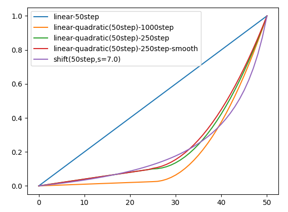
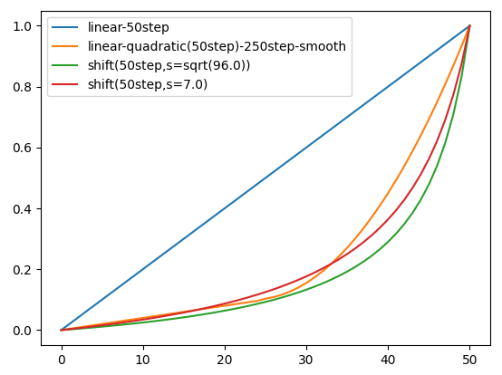
plt.plot(x,y1,label='linear-50step')
plt.plot(x,y2,label='linear-quadratic(50step)-1000step')
plt.plot(x,y3,label='linear-quadratic(50step)-250step')
plt.plot(x,y4,label='linear-quadratic(50step)-250step-smooth')
plt.plot(x,y5,label='shift(50step,s=7.0)')
plt.legend()
plt.show()
論文には実際にはN = 250の線形ステップをエミュレートするのが良いと述べられている。
実のところ少ない推論stepにおいてはこの勾配の大きさは後述のシフト関数s=7のプロットと近く見える。
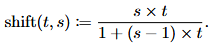
shifting function(Hunyuanvideo)
一方のHunyuanvideoでは以下のようなシフト関数が見られる。
f(t,s)= \frac{s*t}{1+(s-1)*t}
推論が10stepではs=17、推論が50stepではs=7という値があるもののそれ以外の推論stepのsの値の情報はない。
参考までにkohya氏によれば20stepの推奨shiftは14.5と述べられている。
--fs discrete flow shiftを指定します。省略時は14.5で、ステップ数20の場合に対応した値です。HunyuanVideoの論文では、ステップ数50の場合は7.0、ステップ数20未満(10など)で17.0が推奨されています。
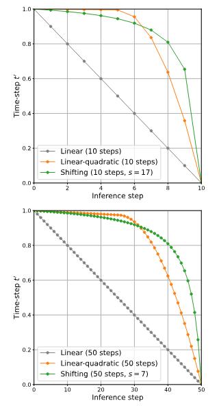
一方、Linear-quadraticの図もあるが25stepで0.025、5stepでは0.005進んでいるように見えるから図は1000stepのエミュレートである。Movie Genは250stepのエミュレートを使ってるとあるので図が正しくないように思う。実際には250stepのエミュレートではシフト関数s=7のプロットとある程度近い。
StableDiffusion3
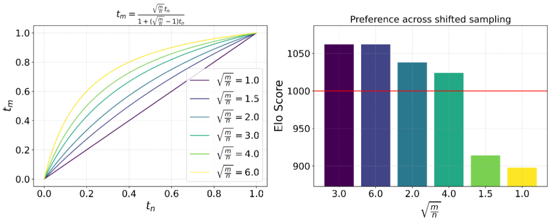
この前述のシフト関数はSD3の論文で既に現れており、この場合は$s=3.0$であった。
しかし、$n$や$m$の値は解像度を示しているようである、Hunyuan Videoとは意味合いが異なるように感じる。
論文には学習、生成それぞれに$s=3.0$のシフトを使用するとある。
Simple Diffusion
SD3の論文内で言及されている論文。
解像度によってタイムステップのシフトが行われている。
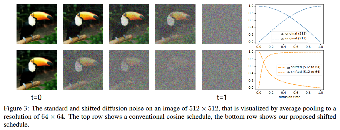
異なる解像度によるシフト関数は以下のようにして求まる。
$\alpha_t=(1-t), \sigma_t=t$の時、
SNR=(\frac{1-t'}{t'})^2=(\frac{1-t}{t})^2\frac{1}{s^2}
(1-t')=\frac{(1-t)}{t}\frac{1}{s}\cdot t'
(\frac{(1-t)}{t}\frac{1}{s}+1)t'=1
t'=\frac{st}{1+(s-1)t}
FasterDiT
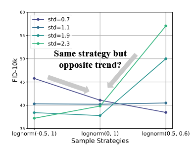
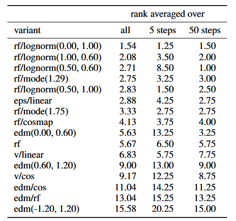
シフト関数は述べられてないが、lognormの設定に関する議論が見られる。7倍学習が高速化するそうだ。
灰色一色の画像と白と黒のグラデーションの画像は平均が同じでも信号偏差が異なるからSNRを一定となるよう加えるノイズに対する信号のばらつきの大きさを調整したいということなのだろうか。
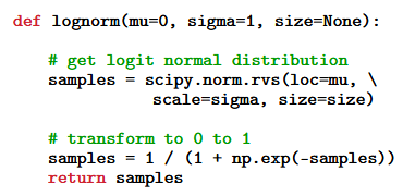
信号対雑音(SNR)確率密度関数(PDF)解析により、DiTのトレーニングプロセスにおける性能とロバスト性のトレードオフを示す。訓練を迅速に行うためには、訓練中に適切なSNRに集中するPDFを持つべきである。...次に、訓練データの標準偏差(std)を調整することで、訓練中に最適なSNRに集中するようにPDFを調整する。さらに、ロジット正規関数[1]を採用し、調整された領域に焦点を絞る。
また、logit-normの計算は正規分布のデータをsigmoid関数に通している。
APT
同じようなシフト関数が見られる。sはlatent次元のh',w',t'によるとある。
実験的に画像の場合はs=1、動画の場合はs=12を使うと書かれている。ただし、このモデルは推論stepが非常に小さい。
(仮説):VAEの圧縮比率
シフト係数がVAEの次元の圧縮比率に依存しているという説。
SD3では生成画像は$(W,H,3)$でlatentは$(W/8,H/8,16)$で考えると3.464となる。
$\sqrt{\frac{8*8*3}{1*1*16}}=\sqrt{12}=3.464$
一方、3D VAEにおける生成動画は$(W,H,T,3)$でlatentは$(W/8,H/8,T/4,16)$で考えると偶然かもしれないが7.0に近い。この仮説はこの値が近いというだけで書いており、理論的な裏付けは全くない。
$\sqrt{\frac{8*8*4*3}{1*1*1*16}}=\sqrt{48}=6.928$
ただ、この理論で行くとMovie Genの生成動画は$(W,H,T,3)$でlatentは$(W/8,H/8,T/8,16)$だから
$\sqrt{\frac{8*8*8*3}{1*1*1*16}}=\sqrt{96}=9.798$となる。
この値($\sqrt{96}$)でも30stepまでのlinear-quadraticとある程度近いように見える。
(仮説):推論stepが少ない場合の倍率
50stepでは$s=7$であるが、10stepでは$s=17$である。このstep比率にルートを掛けた倍率になるという説。この仮説によれば$s=17$は$7*\sqrt{\frac{50}{10}}=7*\sqrt{5}=15.65$である。もっとも特に根拠がある訳ではない。
自分の使ってるHunyuanvideoのワークフローは推論step20であるので、この場合のsの値を考えてみたい。
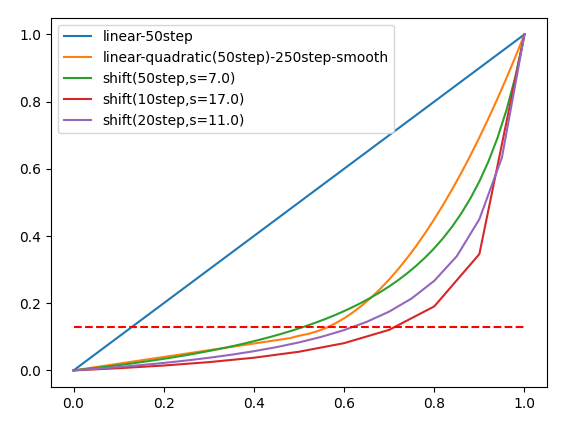
これが仮に20stepにおいて同様に計算できるなら$7*\sqrt{2.5}=11.068$となる。これを試しにプロットしてみると以下のようになる。おおよそ0.13あたりまで線形にすすみ、以降は二次関数的になるという傾向はsの値が異なっても同じである。
一方で推論ステップが初期推論stepにおいて線形になる割合に注目するとs=7では50%、s=11では60%、s=17では70%であり、sが大きいほど多くの割合を初期推論に費やす。
s = 7
a = 1.57
x = np.arange(51)
y1 = np.arange(51)/50
y2 = np.where(x < 25, 0.004 * x, (x-25+a)*(x-25+a)/(25+a)/(25+a)*(1-0.1)+0.1)
y3 = 1-(s * (1-y1))/(1+(s-1)*(1-y1))
plt.plot(x/50,y1,label='linear-50step')
plt.plot(x/50,y2,label='linear-quadratic(50step)-250step-smooth')
plt.plot(x/50,y3,label='shift(50step,s=7.0)')
s = 17
x = np.arange(11)
y1 = np.arange(11)/10
y4 = 1-(s * (1-y1))/(1+(s-1)*(1-y1))
plt.plot(x/10,y4,label='shift(10step,s=17.0)')
x = np.arange(21)
y1 = np.arange(21)/20
s = 11
y5 = 1-(s * (1-y1))/(1+(s-1)*(1-y1))
plt.plot(x/20,y5,label='shift(20step,s=11.0)')
plt.hlines(0.13, 0, 1, colors='red', linestyle='dashed')
plt.legend()
plt.show()
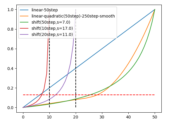
横軸をstep幅を一致させなければ以下のようになる。
stepが少なくなるほど勾配の大きさは先ほどのプロットと異なり初期推論の割合が増えても最初の推論stepの勾配は大きくなる。
s = 7
a = 1.57
x = np.arange(51)
y1 = np.arange(51)/50
y2 = np.where(x < 25, 0.004 * x, (x-25+a)*(x-25+a)/(25+a)/(25+a)*(1-0.1)+0.1)
y3 = 1-(s * (1-y1))/(1+(s-1)*(1-y1))
plt.plot(x,y1,label='linear-50step')
plt.plot(x,y2,label='linear-quadratic(50step)-250step-smooth')
plt.plot(x,y3,label='shift(50step,s=7.0)')
s = 17
x = np.arange(11)
y1 = np.arange(11)/10
y4 = 1-(s * (1-y1))/(1+(s-1)*(1-y1))
plt.plot(x,y4,label='shift(10step,s=17.0)')
x = np.arange(21)
y1 = np.arange(21)/20
s = 11
y5 = 1-(s * (1-y1))/(1+(s-1)*(1-y1))
plt.plot(x,y5,label='shift(20step,s=11.0)')
plt.vlines(10, 0, 1, colors='black', linestyle='dashed')
plt.vlines(20, 0, 1, colors='black', linestyle='dashed')
plt.hlines(0.13, 0, 50, colors='red', linestyle='dashed')
plt.legend()
plt.show()
finetuneのコードのshiftを調べる
diffusion-pipe
        timestep_sample_method = self.model_config.get('timestep_sample_method', 'logit_normal')

        if timestep_sample_method == 'logit_normal':
            dist = torch.distributions.normal.Normal(0, 1)
        elif timestep_sample_method == 'uniform':
            dist = torch.distributions.uniform.Uniform(0, 1)
        else:
            raise NotImplementedError()

        if timestep_quantile is not None:
            t = dist.icdf(torch.full((bs,), timestep_quantile, device=latents.device))
        else:
            t = dist.sample((bs,)).to(latents.device)

        if timestep_sample_method == 'logit_normal':
            sigmoid_scale = self.model_config.get('sigmoid_scale', 1.0)
            t = t * sigmoid_scale
            t = torch.sigmoid(t)

        if shift := self.model_config.get('shift', None):
            t = (t * shift) / (1 + (shift - 1) * t)
...
musubi-tuner
            if args.timestep_sampling == "uniform" or args.timestep_sampling == "sigmoid":
                # Simple random t-based noise sampling
                if args.timestep_sampling == "sigmoid":
                    t = torch.sigmoid(args.sigmoid_scale * torch.randn((batch_size,), device=device))
                else:
                    t = torch.rand((batch_size,), device=device)

            elif args.timestep_sampling == "shift":
                shift = args.discrete_flow_shift
                logits_norm = torch.randn(batch_size, device=device)
                logits_norm = logits_norm * args.sigmoid_scale  # larger scale for more uniform sampling
                t = logits_norm.sigmoid()
                t = (t * shift) / (1 + (shift - 1) * t)
見た感じ、正規分布乱数にシグモイド関数を掛け0~1の変数にしてそれに前述のシフト関数を掛けているだけである。SD3の論文にも正規分布を作って標準logit関数(標準シグモイド関数)を通すとあるので同じだと思われる。
拡散過程と推論過程ではtの進み方が逆だが、一旦それは考えないことにする。
Logit-normal_distribution
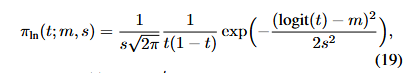
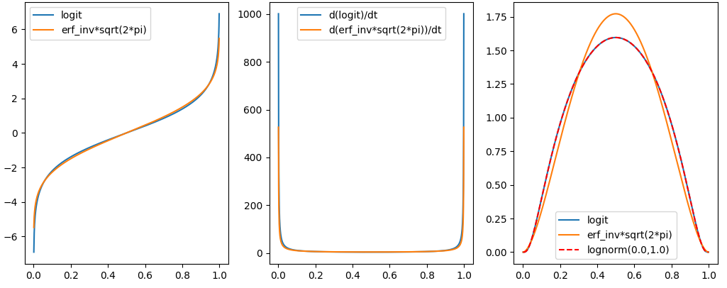
実装コードでは正規分布のデータをsigmoid関数に通して求めるのが簡単だが、ここでは厳密に0~1の一様分布から出発してLogit-normal_distributionに入れ確率密度関数(PDF)を求めることを考えてみたい。
logit(t)=\log{\frac{t}{(1-t)}}=\log{t}-\log{(1-t)}
\frac{d(logit(t))}{dt}=\frac{1}{t}+\frac{1}{1-t}=\frac{1}{t(1-t)}
とはいえlogit関数はerf_inv関数(probit)の近似に過ぎないのであろう。
import numpy as np
import matplotlib.pyplot as plt
from scipy.special import logit, erfinv
from scipy.stats import norm

fig = plt.figure()
ax1 = fig.add_subplot(1, 3, 1)
ax2 = fig.add_subplot(1, 3, 2)
ax3 = fig.add_subplot(1, 3, 3)

t = np.linspace(10e-4, 1-10e-4, 1000)
y1 = logit(t)
y2 = erfinv(t*2-1.0)*np.sqrt(2*np.pi)
y3 = 1/(t*(1-t))
y4 = np.sqrt(2)*np.pi*np.exp(y2**2/(2*np.pi))
y5 = 1/np.sqrt(2*np.pi)*np.exp(-y1**2/2)*y3
y6 = 1/np.sqrt(2*np.pi)*np.exp(-y2**2/2)*y4
y7 = norm.pdf(y1, loc=0.0, scale=1.0)*y3

ax1.plot(t, y1, label='logit')
ax1.plot(t, y2, label='erf_inv*sqrt(2*pi)')
ax2.plot(t, y3, label='d(logit)/dt')
ax2.plot(t, y4, label='d(erf_inv*sqrt(2*pi))/dt')
ax3.plot(t, y5, label='logit')
ax3.plot(t, y6, label='erf_inv*sqrt(2*pi)')
ax3.plot(t, y7, label='lognorm(0.0,1.0)', color='red', linestyle='dashed')
ax1.legend()
ax2.legend()
ax3.legend()
plt.show()
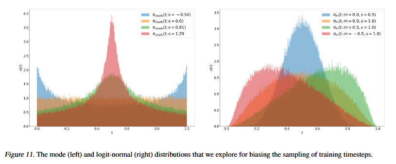
SD3論文よりLogit-normal_distributionの$lognorm(\mu,\sigma)$に$\mu=0$以外の値を与えると非対称に確率密度関数(PDF)はシフトする。この非対称シフトは前述のシフト関数のずれと近い。
プロット
ここでLogit-normal_distributionの求め方に二通りの方法がある。
・正規分布を作成=>シグモイド関数を通す=>シフト関数を通す
・0~1の一様分布tを作成=>Logit-normal_distributionで確率密度関数(PDF)を求める=>tをシフト関数を通す
前者はfinetuneの実装上で見られ、後者は論文式から計算する。
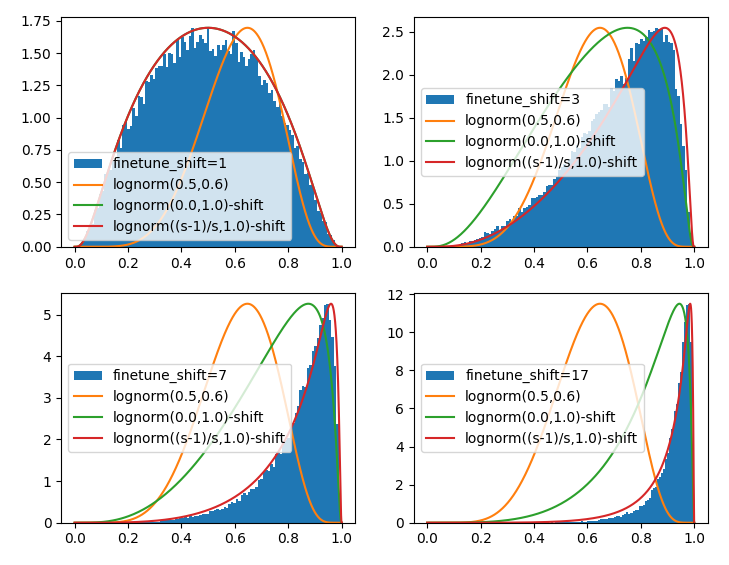
この両者を比較したい。Logit-normal_distributionを参考に適当にplot関数を与えると以下のようになった。ついでにlognorm(0.5,0.6)もplotする
前者と後者はshift=1.0では一致するのだが、shift>1では一致しない。 一致するように調整すると適当に$\mu$の値を動かさなければならないのだが、これがどこからきたのかさっぱり分からない。
import numpy as np
import torch
import matplotlib.pyplot as plt
from scipy.special import logit
from scipy.stats import norm

fig = plt.figure()
ax = []
for i, shift in enumerate([1.0, 3.0, 7.0, 17.0]):
    ax.append(fig.add_subplot(2, 2, i+1))
    x = torch.randn(40000)
    t = torch.sigmoid(x)
    t = (t * shift) / (1 + (shift - 1) * t)
    t = t.to('cpu').detach().numpy()
    ax[i].hist(t, bins=100, density=True, label="finetune_shift=%1.f" % (shift))

#    x = torch.randn(40000)
#    x = 0.5 + x * 0.6
#    t = torch.sigmoid(x)
#    t = (t * shift) / (1 + (shift - 1) * t)
#    t = t.to('cpu').detach().numpy()
#    ax[i].hist(t, bins=100, density=True, label="finetune_(lognorm(0.5,0.6))_shift=%1.f" % (shift))

    hist, bins = np.histogram(t, density=True, bins=100)
    hmax = np.max(hist)

    t = np.linspace(10e-10, 1-10e-10, 1000)
    y = norm.pdf(logit(t), loc=0.5, scale=0.6)/(t*(1-t))
    ax[i].plot(t, y/np.max(y)*hmax, label='lognorm(0.5,0.6)')

    t2 = np.linspace(10e-10, 1-10e-10, 1000)
    y = norm.pdf(logit(t2), loc=0.0, scale=1.0)/(t2*(1-t2))
    t2 = (t2 * shift) / (1 + (shift - 1) * t2)
    ax[i].plot(t2, y/np.max(y)*hmax, label='lognorm(0.0,1.0)-shift')

    t3 = np.linspace(10e-10, 1-10e-10, 1000)
    y = norm.pdf(logit(t3), loc=np.sqrt(2/np.pi)*(shift-1)/shift, scale=1.0)/(t3*(1-t3))
    t3 = (t3 * shift) / (1 + (shift - 1) * t3)
    ax[i].plot(t3, y/np.max(y)*hmax, label='lognorm((s-1)/s,1.0)-shift')

    plt.legend()
plt.show()
まとめ
shifting factorについて調べた。良い値をとればDiTの学習が効率的になる(または推論stepが小さい時の精度が良くなる)らしいが、どの値が良いのかというのはバラバラだった。SD3ではs=3、HunyuanVideo 50stepではs=7.0、10stepではs=17.0、APTでは画像でs=1、動画でs=12、diffusion-pipeのhunyuanvideoではs=7.0、Musubi-tunerではs=7.0かs=3.0、Movie Genだとlinear-quadraticを用いるが250stepのエミュレートでは実質s=7~10くらいが近い。
SD3では論文中例えば、幅と高さを2倍にすると、任意の時間0 < t < 1において不確実性が半分になることがすぐにわかります。とあるので$\sqrt{\frac{m}{n}}$は学習と推論の画像の解像度を議論していると思われる。Movie Genでは動画生成の最初の推論stepの影響が大きいのを示し、推論stepの前半半分をN=250step相当の線形移動にして(慎重に動き)、後半は二次関数で一気に動く。Hunyuan Videoにおいては50stepより推論stepが更に小さいとshiftを更に大きくした方が良い事を示されている。これは慎重に動く割合を推論step全体の前半50%から前半70%にすると理解される。FasterDiTはあまり読めてないのだが、学習画像の信号のばらつきを等しくしようとしている。APTではshiftはlatentの解像度だけでなくフレーム方向の次元に依存し、画像と動画で異なるshiftを採用する。
と論文の議論の方向性もばらばらでlatent次元だったり、学習データのばらつきの大きさだったり、初期推論stepの慎重性だったり、低推論stepの最適値だったり、学習の効率性だったり、シフト関数ではなくlognormやlinear-quadraticを議論してたりで統一性も見られない。