一般にBitNetの量子化では1bit量子化などの対象は正負で対称な行列である。
$W$の符号が正の部分と負の部分で分布が異なる場合、$\alpha,\beta$が平均値では上手く決定できないのではと考えた。
例えば4分割の量子化を以下の様に与えたとする。
\alpha = mean(W)
\beta= mean(abs(W-\alpha))
qW = \beta * (clip(round(\frac{W-\alpha}{\beta}+1.5),0,3)-1.5)
下記のように範囲によって分布が異なる時($W>0.0$で2倍)、このような非対称の分布がある場合、上述の$\alpha,\beta$をnp.percentileおよびscipy.interpolate.interp1dを使って係数を求めてみたい。
W = np.random.randn(360, 768)
Wasym = np.where(W>0.0, W*2.0, W)
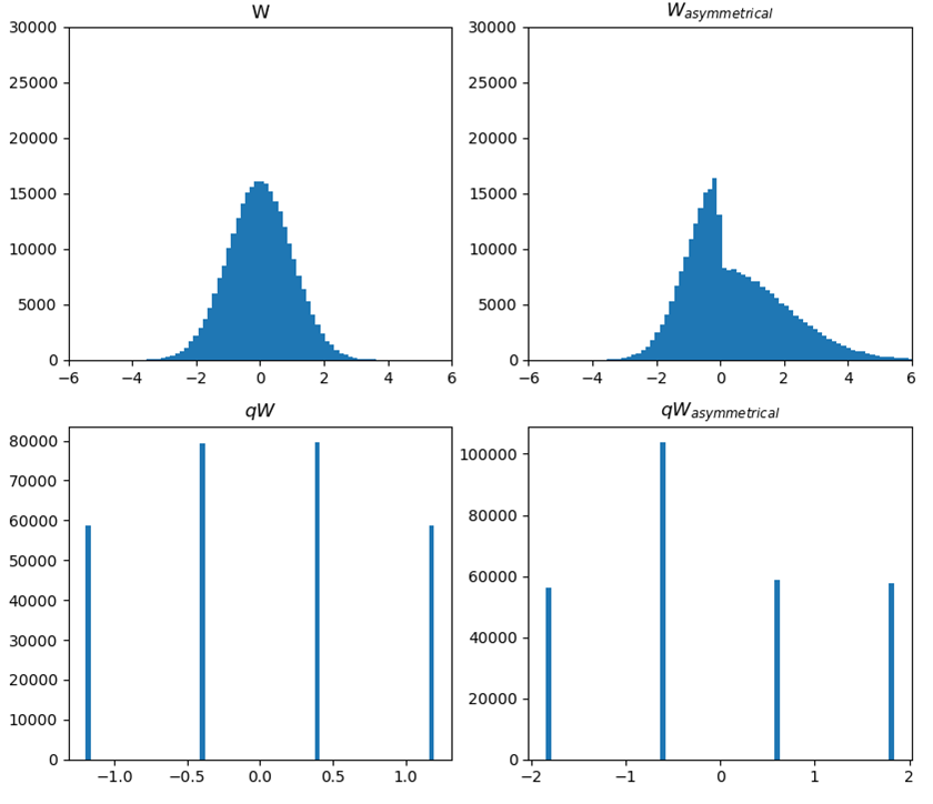
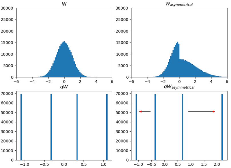
等4分割(bit2)
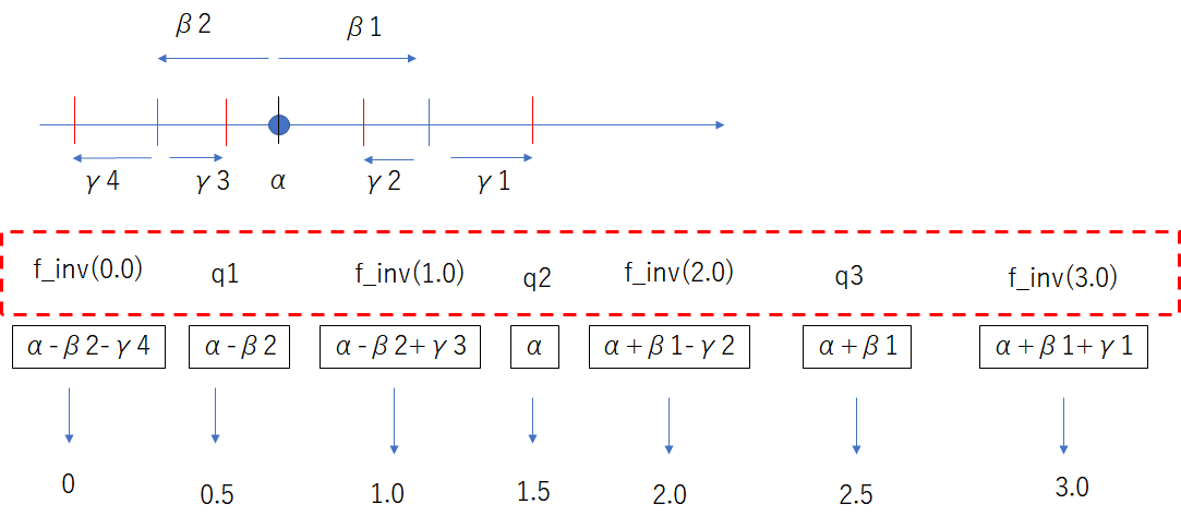
四分位数を求め、それらが0.5,1.5,2.5となる変換関数$f(x)$を求め、この変換関数後の値を量子化する$W_2=clip(round(f(W)))$。更にfの逆変換関数を掛け、$qW=f_{inv}(W_2)$求める。
何故変換先の値が0.5,1.5,2.5となるようにしているかというとround関数(四捨五入関数)の値の切り替わりが整数の中間になるようにである。
この場合の量子化の値は$f_{inv}(0.0),f_{inv}(1.0),f_{inv}(2.0),f_{inv}(3.0)$に変換される。
def quant2(W, kind='linear'):
    orig_shape = W.shape
    q1 = np.percentile(W.flatten(), 25)
    q2 = np.percentile(W.flatten(), 50)
    q3 = np.percentile(W.flatten(), 75)
    qmin = np.percentile(W.flatten(), 1)
    qmax = np.percentile(W.flatten(), 99)

    W2 = np.clip(W, qmin, qmax).flatten()
    x = [qmin, q1, q2, q3, qmax]
    y = [-2.32/0.798+1.5, 0.5, 1.5, 2.5, 2.32/0.798+1.5]

    f = scipy.interpolate.interp1d(x, y, kind=kind)
    f_inv = scipy.interpolate.interp1d(y, x, kind=kind)

    W2 = np.clip(np.round(f(W2)),0, 3)
    qW = f_inv(W2).reshape(orig_shape)
    return qW
この時、分布が非対称の場合においても等しく分割する事が可能である。
また、その時の間隔も正と負で異なる間隔で刻むことが可能である。
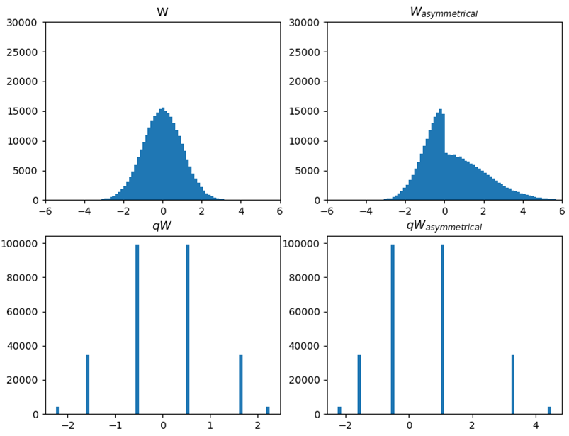
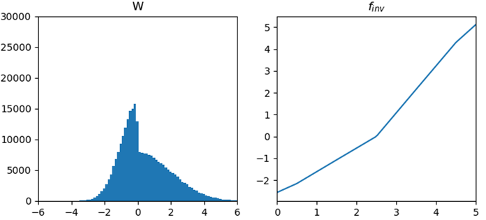
非等6分割(bit2)
とはいえこのような出現確率が等分の量子化が良いかというと決してそんなことは無く、大きな値の再現度がいまいちのためかcos類似度で見ると良くない。
例えば下記の6分割はエントロピー的には$(0.0155*log2(0.0155)+0.1250*log2(0.1250)+0.3595*log2(0.3595))*2=1.998bit$であり、等分割の4分割(2bit相当)の分割とエントロピーは変わらない。
にもかかわらず、演算結果のcos類似度で観察すると前述の等分割の4分割より優秀である。
def quant3(W, kind='linear'):
    orig_shape = W.shape
    q1 = np.percentile(W.flatten(), 1.55)
    q2 = np.percentile(W.flatten(), 14.05)
    q3 = np.percentile(W.flatten(), 50.00)
    q4 = np.percentile(W.flatten(), 85.95)
    q5 = np.percentile(W.flatten(), 98.45)
    qmin = np.percentile(W.flatten(), 0.5)
    qmax = np.percentile(W.flatten(), 99.5)

    W2 = np.clip(W, qmin, qmax).flatten()
    x = [qmin, q1, q2, q3, q4, q5, qmax]
    y = [0.0, 0.5, 1.5, 2.5, 3.5, 4.5, 5.0]

    f = scipy.interpolate.interp1d(x, y, kind=kind)
    f_inv = scipy.interpolate.interp1d(y, x, kind=kind)

    W2 = np.clip(np.round(f(W2)), 0, 5)
    qW = f_inv(W2).reshape(orig_shape)
    return qW
なお$1.55$とか$14.05$とかの係数は割と適当であり、エントロピー2bit以下でcos類似度の最大値を取る最適値の探索もやってみたのだがcos類似度の収束は与えた$W$に依存するので係数の同定は出来なかった。
おおよそq1は1.2~2.2%、q2は13~16%、qminは0.15~0.6%ぐらいで最適値をとるが、cos類似度の差は例えばある重みでは探索しない場合(quant3)で0.944、探索して0.949なので探索する価値はそれほどない。
def quant4(W, kind='linear', p1=0.5, p2=1.55, p3=14.05):
    orig_shape = W.shape
    q1 = np.percentile(W.flatten(), p2)
    q2 = np.percentile(W.flatten(), p3)
    q3 = np.percentile(W.flatten(), 50.00)
    q4 = np.percentile(W.flatten(), 100-p3)
    q5 = np.percentile(W.flatten(), 100-p2)
    qmin = np.percentile(W.flatten(), p1)
    qmax = np.percentile(W.flatten(), 100-p1)

    W2 = np.clip(W, qmin, qmax).flatten()
    x = [qmin, q1, q2, q3, q4, q5, qmax]
    y = [0.0, 0.5, 1.5, 2.5, 3.5, 4.5, 5.0]

    f = scipy.interpolate.interp1d(x, y, kind=kind)
    f_inv = scipy.interpolate.interp1d(y, x, kind=kind)

    W2 = np.clip(np.round(f(W2)), 0, 5)
    qW = f_inv(W2).reshape(orig_shape)
    entropy = 0.0
    for i in range(6):
        rate = np.count_nonzero(W2==i)/len(W2)
        entropy += -rate*np.log2(rate)
    return qW, entropy
この場合の$f_{inv}$は正負で傾きの異なる単なる折れ線グラフである。
この折れ線は([0.0, 0.5, 1.5, 2.5, 3.5, 4.5, 5.0], [qmin, q1, q2, q3, q4, q5, qmax])を必ず通る。
もし0.5%や1.55%の外れ値に信頼が置けないなら、下記のようにすれば外れ値に左右されずに変換関数を求められるが、絶対値の大きさの範囲によって途中で分散が変わる分布ではエントロピーが分布に依存し、事前に決定できない。
    q2 = np.percentile(W.flatten(), 14.05)
    q3 = np.percentile(W.flatten(), 50.00)
    q4 = np.percentile(W.flatten(), 85.95)
    q1 = q3 + (q2-q3)*2.0
    q5 = q3 + (q4-q3)*2.0
    qmin = q3 + (q2-q3)*3.0
    qmax = q3 + (q4-q3)*3.0

    W2 = np.clip(W, qmin, qmax).flatten()
    x = [qmin, q1, q2, q3, q4, q5, qmax]
    y = [-0.5, 0.5, 1.5, 2.5, 3.5, 4.5, 5.5]
まとめ
非対称分布においての分割にnp.percentileおよびscipy.interpolate.interp1dを用いて$\alpha,\beta$の代わりを求める方法を考察した。
エントロピー上は2bitに相当する非等分割の6分割で量子化割した方が等分割の4分割の2bitより良い結果が得られる。
最初は下記のように正と負で異なる$\beta_1,\beta_2$を仮定したり、$\alpha$を求めるのに平均値ではなく中央値を採用したりとか考えたが、やがてnp.percentileを使った計算に落ち着いた。