Kaggleにおいてデータを無作為にサブミットして結果からテストデータの正解ラベルを調べたりすれば機械学習など行わなくてもスコアが$100%$が出るのではないか。おそらく、そんなことは誰もが一度くらいは考えたことがあるのではないでしょうか。
正例か負例を当てる$2$値分類問題でテストデータが$1024$件の場合において、正解ラベルを得るために必要なサブミット回数を考えてみました。
Mastermind問題
Mastermindとは別名ヒット&ブローなどと呼ばれているゲームの種類で隠された球の色と場所をヒット(場所と色が一致)やブロー(色のみ一致)の情報から当てていくゲームである。
有名なMastermindの問題は6色4スロットの問題でKnuthによれば最悪の場合でも5手で全ての球の色と場所が特定できる。
一般に$K$色$N$スロットのMastermindのエントロピー下限は$O(Nlog_{2}K/log_{2}N)$で与えられる。
ところで正解位置であるヒット(場所と色が一致)は多分類におけるKaggleのサブミット結果の点数である。また、ブロー(色の一致情報)は予め統一ラベル(全部同じラベル)でのテスト結果を見ればテスト結果の一致しないラベルの数(ブローの数)は最大一致ラベル数-ヒット数で分かる。
従って、$K$値分類問題のテストデータが$N$個ある場合の正解データを得るためのサブミット回数の見積もりは$K$色$N$スロットのMastermind問題を解くことと等価である。
今回の場合は2値分類問題の場合を考えたいから2色Mastermind問題を考えればよい。
これは古くは1960年に「偽物のコインは9グラム、本物のコインはすべて10グラムです。 組成のわからないコインと、天秤ではなく正確な秤が与えられた場合、偽造コインを分離するためには、何回の計量が必要でしょうか?」という形で議論された。
勿論、$N$枚のコインの真偽を確認するためには、単純に考えれば1枚ずつ$N$回計量すれば全てコインの真偽は分かる。しかし、$N=4$より大きい場合、$N$回を下回る方法が存在する。
これは2色Mastermind問題で$O(N/log_{2}N)$で得られる。$N=1024$では$log_{2}N=10$より
\frac{N}{log_{2}N}=\frac{1024}{10}=102.4
である。
参考論文ではテストデータを同定するまでに必要な回数は$N/log_{2}N$の$α$倍であり、$α$の値は$2≦α≦log_2{9}(3.17)$の範囲にあることが述べられている。
すなわち、理論的には$N=1024$で必要なサブミット回数は$200~320$と見積もられる。
ただ、どういう議論でこれが導き出されたかについては理解してない。
次に実際にプログラムを書いてみてサブミット回数を考えてみたい。
解1.N回(1024回)
一番最初に1bitずつチェックしていく手法を考える。
注意すべきはプログラム上ではチェックしたい範囲を選択できるのだが、実際のサブミットでは特定の範囲を指定してテスト結果を返すことができない。(全てのbitがチェックされる)
従って実際のサブミットにおいては結果をチェックしない範囲には0.5を代入すれば、テストデータの正解が正例でも負例でも同じ結果を返すから結果から0.5を入れた数のスコアを差し引けば、特定の範囲を指定したと考えるテスト結果を得る事ができる。
この0.5を代入する作業は省略するとして、1bitずつチェックする範囲を指定すれば$N=1024$のデータは$1024$回で同定できる。
import numpy as np

def test(y_pred, y_true):
    return len(y_pred) - np.sum(np.abs(y_pred - y_true))

def Solve1(length): # N
    global iter
    y_check = np.array([1] * int(1))
    for index in range(length):
        result = test(y_check, y_true[index])
        iter += 1
        if result == 1:
            y_pred[index] = 1
n = 1024
iter = 0
y_pred = np.array([0] * n)
y_true = np.random.randint(0, 2, (n))
Solve1(1024)
print(iter, y_pred, y_true, test(y_pred, y_true))
---------------------------------------
1024 [0 0 0 ... 0 1 1] [0 0 0 ... 0 1 1] 1024
解2.3/4*N回(768回)
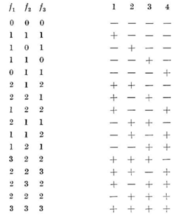
偽造コインの真偽を確認する問題で示されるように4bit毎に3回のチェックで同定する手法がある。
例えば4枚のコイン1,2,3,4に対して
f1:コイン1,2,3を計る
f2:コイン1,3,4を計る
f3:コイン1,2,4を計る
の結果を比較すれば3回の測定結果から4枚のコインの真偽について同定できる。
従ってコインが4の倍数なら$N=4m$の場合、4枚ずつ同定していけば$3m$回で全てのコインを同定できる。
import numpy as np

def test(y_pred, y_true):
    return len(y_pred) - np.sum(np.abs(y_pred - y_true))

def Solve2(length): # N * 3/4
    global iter
    y_check = np.array([1] * int(3))
    for index in range(0,length,4):
        result1 = test(y_check, y_true[[index, index+1, index+2]])
        result2 = test(y_check, y_true[[index, index+2, index+3]])
        result3 = test(y_check, y_true[[index, index+1, index+3]])
        result = (result1,result2,result3)
        iter += 3

        if result==(0,0,0):
            y_pred[index:index+4] = 0
        if result==(1,1,1):
            y_pred[index] = 1
        if result==(1,0,1):
            y_pred[index+1] = 1
        if result==(1,1,0):
            y_pred[index+2] = 1
        if result==(0,1,1):
            y_pred[index+3] = 1
        if result==(2,1,2):
            y_pred[index] = 1
            y_pred[index+1] = 1
        if result==(2,2,1):
            y_pred[index] = 1
            y_pred[index+2] = 1
        if result==(1,2,2):
            y_pred[index] = 1
            y_pred[index+3] = 1
        if result==(2,1,1):
            y_pred[index+1] = 1
            y_pred[index+2] = 1
        if result==(1,1,2):
            y_pred[index+1] = 1
            y_pred[index+3] = 1
        if result==(1,2,1):
            y_pred[index+2] = 1
            y_pred[index+3] = 1
        if result==(3,2,2):
            y_pred[index] = 1
            y_pred[index+1] = 1
            y_pred[index+2] = 1
        if result==(2,2,3):
            y_pred[index] = 1
            y_pred[index+1] = 1
            y_pred[index+3] = 1
        if result==(2,3,2):
            y_pred[index] = 1
            y_pred[index+2] = 1
            y_pred[index+3] = 1
        if result==(2,2,2):
            y_pred[index+1] = 1
            y_pred[index+2] = 1
            y_pred[index+3] = 1
        if result==(3,3,3):
            y_pred[index:index+4] = 1

n = 1024
iter = 0

y_pred = np.array([0] * n)
y_true = np.random.randint(0, 2, (n))
Solve2(1024)
print(iter, y_pred, y_true, test(y_pred, y_true))
---------------------------------------
768 [1 0 1 ... 1 0 1] [1 0 1 ... 1 0 1] 1024
解3.735回
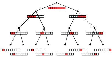
例えば最初に1~1024bit調べ、次に1~512bitを調べるとする。
この時、513~1024bitの結果は(1~1024bitの結果 - 1~512bitの結果)で計算できる。次に1~256bitを調べると257~512bitの結果は(1~512bitの結果 - 1~256bitの結果)で計算できる。
このように上位からチェックbitを半分にしつつチェックしていけば愚直には$1+1+2+4+8+…+256+512=1024$回で全てのbitを確定できる。この操作自体は別にトータルのチェック回数を減らせるわけではない。
この時、1024bitのチェックは1回行い、512bitのチェックは1回行い、256bitのチェックは2回行い、…4bitのチェックは128回行い、2bitのチェックは256回行い、1bitのチェックは512回行う。
4bitの結果が$0,4$の場合はその時点で$(0,0,0,0),(1,1,1,1)$である事が同定されるので下位bitはチェックしなくてよい。4bitのチェックは約$1/8$の確率で以降のチェックを3回減らせる。
同様に2bitの結果が$0,2$の場合はその時点で$(0,0),(1,1)$である事が同定されるので下位bitはチェックしなくてよい。2bitのチェックは約$1/2$の確率で以降のチェックを1回減らせる。
この省略できる度合いは確率に依存するため実行毎に結果が異なるが、平均すると735回程度である。
このような手法は適応戦略(adaptive strategy)であり、サブミット回数はテストデータの偏りに依存する。一方、解2は非適応戦略(non-adaptive strategy)でサブミット回数はテストデータの偏りに依存しない。
import numpy as np

def test(y_pred, y_true):
    return len(y_pred) - np.sum(np.abs(y_pred - y_true))

def comit(y_true, index, length):
    global iter
    y_check = np.array([1] * int(length))
    result = test(y_check, y_true[index:index+length])
    iter += 1
    return result

def input_data(y_pred, index, length, result):
    if result == 0:
        y_pred[index:index+length] = 0
    elif result == length:
        y_pred[index:index+length] = 1

def check(index, length, upper_result):
    result = comit(y_true, index, length)

    if result in [0,length]:
        input_data(y_pred, index, length, result)
    else:
        check(index, length//2, result)

    if upper_result is None:
        return

    index += length
    result2 = upper_result - result
    if result2 in [0,length]:
        input_data(y_pred, index, length, result2)
    else:
        check(index, length//2, result2)

def Solve3(length):
    check(0, length, None)

n = 1024
iter = 0
y_pred = np.array([0] * n)
y_true = np.random.randint(0, 2, (n))
Solve3(1024)
print(iter, y_pred, y_true, test(y_pred, y_true))
---------------------------------------
735 [1 1 0 ... 1 0 0] [1 1 0 ... 1 0 0] 1024
解2A.21/32*N回(672回)
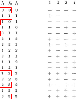
もう一度、4bit毎に確認する方法をチェックするとf1,f2,f3の3回チェックする必要があるが、f1またはf2が$0,3$の場合はf1,f2の2回チェックで4bitを同定できる。
$6/16$の確率でチェック2回で4bitを同定でき、$10/16$の確率でチェック3回で4bitを同定できるから、期待値は$6/162/4+10/163/4=42/64=21/32$である。
def Solve2A(length): # N * 21/32
    global iter
    y_check = np.array([1] * int(3))
    for index in range(0,length,4):
        result1 = test(y_check, y_true[[index, index+1, index+2]])
        result2 = test(y_check, y_true[[index, index+2, index+3]])
        result = (result1,result2)
        iter += 2

        if result[0] in [0,3] or result[1] in [0,3]:
            if result==(0,0):
                y_pred[index:index+4] = 0
            if result==(1,0):
                y_pred[index+1] = 1
            if result==(0,1):
                y_pred[index+3] = 1
            if result==(3,2):
                y_pred[index] = 1
                y_pred[index+1] = 1
                y_pred[index+2] = 1
            if result==(2,3):
                y_pred[index] = 1
                y_pred[index+2] = 1
                y_pred[index+3] = 1
            if result==(3,3):
                y_pred[index:index+4] = 1
        else:
            result3 = test(y_check, y_true[[index, index+1, index+3]])
            result = (result1,result2,result3)
            iter += 1

            if result==(1,1,1):
                y_pred[index] = 1
            if result==(1,1,0):
                y_pred[index+2] = 1
            if result==(2,1,2):
                y_pred[index] = 1
                y_pred[index+1] = 1
            if result==(2,2,1):
                y_pred[index] = 1
                y_pred[index+2] = 1
            if result==(1,2,2):
                y_pred[index] = 1
                y_pred[index+3] = 1
            if result==(2,1,1):
                y_pred[index+1] = 1
                y_pred[index+2] = 1
            if result==(1,1,2):
                y_pred[index+1] = 1
                y_pred[index+3] = 1
            if result==(1,2,1):
                y_pred[index+2] = 1
                y_pred[index+3] = 1
            if result==(2,2,3):
                y_pred[index] = 1
                y_pred[index+1] = 1
                y_pred[index+3] = 1
            if result==(2,2,2):
                y_pred[index+1] = 1
                y_pred[index+2] = 1
                y_pred[index+3] = 1
解4.10/16*N回(640回)
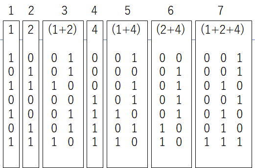
4bit毎に3回確認する方法では3回のチェックするbitは$(1,1,1,0),(1,1,0,1),(1,0,1,1)$の三通りの結果がそれぞれ得られる。この三回の結果を足すと$(3,2,2,2)$の結果が得られる。これを2で割った時の商が$(1,1,1,1)$、余りは$(1,0,0,0)$である。商の結果$(1,1,1,1)$から各チェックの結果を差し引けば$(0,0,0,1),(0,0,1,0),(0,1,0,0)$が得られる。
要するに解2では16通りの場合分けを全て考えていたが、結果の総和の商や余りを演算することによって場合分け(if文分岐)を考えずとも同定可能である。
では、以下の様な16bit毎に9回チェックを行う方法を考え、これの結果の総和の商や余りを演算することでbitを同定したい。実はこれは4bit毎に3回確認する方法を2回複合したような形である。計算手順の都合により1回余計なチェックが挿入されているため16bit毎に10回チェックが必要になっているが、少なくとも条件分岐(bit全探索)を考えるよりも演算量を押さえて地道に同定出来ている。チェック回数の効率も解4は10/16で、解2Aは21/32だから4bitずつ同定するより効率が良い。
import numpy as np

def test(y_pred, y_true):
    return len(y_pred) - np.sum(np.abs(y_pred - y_true))

def Solve4(length): # N * 10/16
    global iter
    y_check = np.array([1] * int(9))
    for index in range(0,length,16):
        result1 = test(y_check, y_true[[index, index+1, index+2, index+4, index+5,  index+6,  index+8,  index+9,  index+10]]) # abc efg ijk
        result2 = test(y_check, y_true[[index, index+1, index+2, index+8, index+9,  index+10, index+12, index+13, index+14]]) # abc ijk mno
        result3 = test(y_check, y_true[[index, index+1, index+2, index+4, index+5,  index+6,  index+12, index+13, index+14]]) # abc efg mno
        result4 = test(y_check, y_true[[index, index+2, index+3, index+4, index+6,  index+7,  index+8,  index+10, index+11]]) # acd egh ikl
        result5 = test(y_check, y_true[[index, index+2, index+3, index+8, index+10, index+11, index+12, index+14, index+15]]) # acd ikl mop
        result6 = test(y_check, y_true[[index, index+2, index+3, index+4, index+6,  index+7,  index+12, index+14, index+15]]) # acd egh mop
        result7 = test(y_check, y_true[[index, index+1, index+3, index+4, index+5,  index+7,  index+8,  index+9,  index+11]]) # abd efh ijl
        result8 = test(y_check, y_true[[index, index+1, index+3, index+8, index+9,  index+11, index+12, index+13, index+15]]) # abd ijl mnp
        result9 = test(y_check, y_true[[index, index+1, index+3, index+4, index+5,  index+7,  index+12, index+13, index+15]]) # abd efh mnp
        result10 = test(y_check[:4], y_true[[index, index+1, index+2, index+3]])                                              # abcd
        print(result1, result2, result3, result4, result5, result6, result7, result8, result9, result10)
        iter += 10

        r00 = result1 + result2 + result3 + result4 + result5 + result6 + result7 + result8 + result9 - result10 * 2 # a+2*(3a+2b+2c+2d + 3e+2f+2g+2h + 3i+2j+2k+2l + 3m+2n+2o+2p)

        a = np.array([1] * int(16))
        a[0] = r00 % 2 # a
        r11 = (r00 // 2 - (result1 + result4 + result7)) # 3m+2n+2o+2p
        r12 = (r00 // 2 - (result2 + result5 + result8)) # 3e+2f+2g+2h
        r13 = (r00 // 2 - (result3 + result6 + result9)) # 3i+2j+2k+2l

        a[4]  = r12 % 2 # e
        a[8]  = r13 % 2 # i
        a[12] = r11 % 2 # m

        r21 = (result10 + r12//2 + r13//2) - result1 # d h l
        r22 = (result10 + r11//2 + r13//2) - result2 # d l p
        r23 = (result10 + r11//2 + r12//2) - result3 # d h p
        r24 = r21 + r22 + r23                        # d+2*(d+h+l+p)

        a[3]  = r24 % 2      # d
        a[7]  = r24//2 - r22 # h
        a[11] = r24//2 - r23 # l
        a[15] = r24//2 - r21 # p

        r31 = (result10 + r12//2 + r13//2) - result4 # b f j
        r32 = (result10 + r11//2 + r13//2) - result5 # b j n
        r33 = (result10 + r11//2 + r12//2) - result6 # b f n
        r34 = r31 + r32 + r33                        # b+2*(b+f+j+n)
        a[1]  = r34 % 2      # b
        a[5]  = r34//2 - r32 # f
        a[9]  = r34//2 - r33 # j
        a[13] = r34//2 - r31 # n

        r41 = (result10 + r12//2 + r13//2) - result7 # c g k
        r42 = (result10 + r11//2 + r13//2) - result8 # c k o
        r43 = (result10 + r11//2 + r12//2) - result9 # c g o
        r44 = r41 + r42 + r43                        # c+2*(c+g+k+o)
        a[2]  = r44 % 2      # c
        a[6]  = r44//2 - r42 # g
        a[10] = r44//2 - r43 # k
        a[14] = r44//2 - r41 # o
        y_pred[index:index+16] = a

n = 1024
iter = 0
y_pred = np.array([0] * n)
y_true = np.random.randint(0, 2, (n))
Solve4(1024)
print(iter, y_pred, y_true, test(y_pred, y_true))
---------------------------------------
640 [0 0 0 ... 1 1 0] [0 0 0 ... 1 1 0] 1024
解5.(27+α)/64*N回?
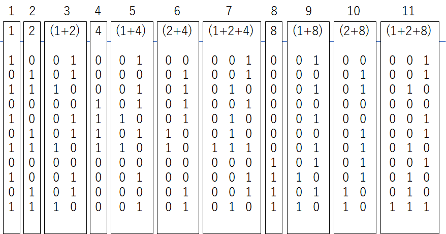
解4は16bit毎に(9+1)回チェックを行う方法で解けることを示した。これは4bit毎に3回チェックする方法を2回複合したような形である。
同じような類推を用いれば64bit毎に27+α回、256bit毎に81+β回、1024bit毎に273+γ回のチェックで解けるのではないかと推定される。
このように求めていければチェック回数をおおよそ3/4ずつ減らしていけるのではと考え、64bit毎の場合に27+α回で解けるか考えてみたのだが、非常に式が複雑で断念した。
解6.7/12*N回(598回)
ある論文に12bitを7回のチェックで同定できる事が示唆されている。ここで7/12は解4の10/16よりも小さい。(14/24と15/24)
ぶっちゃけて言えば論文に書いてある理論の理屈は理解できないのだが、7回のチェックの結果で12bit(4096通り)が作り出せればこのチェックは12bitを同定するチェックだという事が出来る。

例えば以下の様な重み配列を与えた場合、確かに結果は重複無しで4096通りが作り出せる。
def Solve6(length):
    global iter
    rusult_list = []
    for i in range(2**12):

        y_t = np.array(list(format(i, '012b'))).astype('int64')
        y_check = np.array([1] * int(12))
        index = 0
        result1 = test(y_check[:4], y_t[[index, index+3, index+6, index+11]])
        result2 = test(y_check[:4], y_t[[index+1, index+3, index+8, index+11]])
        result3 = test(y_check[:6], y_t[[index, index+1, index+2, index+6, index+8, index+10]])
        result4 = test(y_check[:4], y_t[[index+4, index+6, index+8, index+11]])
        result5 = test(y_check[:6], y_t[[index, index+3, index+4, index+5, index+8, index+10]])
        result6 = test(y_check[:6], y_t[[index+1, index+3, index+4, index+6, index+7, index+10]])
        result7 = test(y_check[:9], y_t[[index, index+1, index+2, index+4, index+5, index+7, index+9, index+10, index+11]])
        result = (result1, result2, result3, result4, result5, result6, result7)
        rusult_list.append(result)

    print(len(rusult_list))
    print(len(set(rusult_list)))

    for index in range(0,1020,12):
        result1 = test(y_check[:4], y_true[[index, index+3, index+6, index+11]])
        result2 = test(y_check[:4], y_true[[index+1, index+3, index+8, index+11]])
        result3 = test(y_check[:6], y_true[[index, index+1, index+2, index+6, index+8, index+10]])
        result4 = test(y_check[:4], y_true[[index+4, index+6, index+8, index+11]])
        result5 = test(y_check[:6], y_true[[index, index+3, index+4, index+5, index+8, index+10]])
        result6 = test(y_check[:6], y_true[[index+1, index+3, index+4, index+6, index+7, index+10]])
        result7 = test(y_check[:9], y_true[[index, index+1, index+2, index+4, index+5, index+7, index+9, index+10, index+11]])
        result = (result1, result2, result3, result4, result5, result6, result7)
        iter += 7
        i = rusult_list.index(result)
        y_pred[index:index+12] = np.array(list(format(i, '012b'))).astype('int64')
---------------------------------------
4096
4096
595 [1 0 0 ... 0 0 0] [1 0 0 ... 1 1 1] 1021
解7.11/20*N回(564回)
同様に20bitを11回のチェックで同定できる。しかし、この時点で分岐の配列を作ろうとすると440MB近く消費してメモリ消費量が目立ってくるし、実行時間も問題で$2^{20}=1048576$通りを全て書き出すのにも非常に時間がかかってしまう(数分かかる)。これの更に一個上12/22(559回)は4倍実行時間とメモリ消費する上に回数削減効果はあまり効果はない。さらに上は13/25(533回)、14/28(514回)はそれぞれ実行時間とメモリ消費が解7の32倍、256倍使われる為、bit全探索の場合分けの配列を作ってやろうとするのは現実的ではない。
def Solve7(length):
    global iter
    rusult_list = []
    for i in range(2**20):

        y_t = np.array(list(format(i, '020b'))).astype('int64')
        y_check = np.array([1] * int(12))
        index = 0
        result1 = test(y_check[:6], y_t[[index, index+3, index+6, index+11, index+14, index+19]])
        result2 = test(y_check[:6], y_t[[index+1, index+3, index+8, index+11, index+16, index+19]])
        result3 = test(y_check[:9], y_t[[index, index+1, index+2, index+6, index+8, index+10, index+14, index+16, index+18]])
        result4 = test(y_check[:4], y_t[[index+4, index+6, index+8, index+11]])
        result5 = test(y_check[:8], y_t[[index, index+3, index+4, index+5, index+8, index+10, index+14, index+19]])
        result6 = test(y_check[:8], y_t[[index+1, index+3, index+4, index+6, index+7, index+10, index+16, index+19]])
        result7 = test(y_check[:12], y_t[[index, index+1, index+2, index+4, index+5, index+7, index+9, index+10, index+11, index+14, index+16, index+18]])
        result8 = test(y_check[:4], y_t[[index+12, index+14, index+16, index+19]])
        result9 = test(y_check[:8], y_t[[index, index+3, index+6, index+11, index+12, index+13, index+16, index+18]])
        result10 = test(y_check[:8], y_t[[index+1, index+3, index+8, index+11, index+12, index+14, index+15, index+18]])
        result11 = test(y_check[:12], y_t[[index, index+1, index+2, index+6, index+8, index+10, index+12, index+13, index+15, index+17, index+18, index+19]])
        result = (result1, result2, result3, result4, result5, result6, result7, result8, result9, result10, result11)
        rusult_list.append(result)

    print(len(rusult_list))
    print(len(set(rusult_list)))

    for index in range(0,1020,20):
        result1 = test(y_check[:6], y_true[[index, index+3, index+6, index+11, index+14, index+19]])
        result2 = test(y_check[:6], y_true[[index+1, index+3, index+8, index+11, index+16, index+19]])
        result3 = test(y_check[:9], y_true[[index, index+1, index+2, index+6, index+8, index+10, index+14, index+16, index+18]])
        result4 = test(y_check[:4], y_true[[index+4, index+6, index+8, index+11]])
        result5 = test(y_check[:8], y_true[[index, index+3, index+4, index+5, index+8, index+10, index+14, index+19]])
        result6 = test(y_check[:8], y_true[[index+1, index+3, index+4, index+6, index+7, index+10, index+16, index+19]])
        result7 = test(y_check[:12], y_true[[index, index+1, index+2, index+4, index+5, index+7, index+9, index+10, index+11, index+14, index+16, index+18]])
        result8 = test(y_check[:4], y_true[[index+12, index+14, index+16, index+19]])
        result9 = test(y_check[:8], y_true[[index, index+3, index+6, index+11, index+12, index+13, index+16, index+18]])
        result10 = test(y_check[:8], y_true[[index+1, index+3, index+8, index+11, index+12, index+14, index+15, index+18]])
        result11 = test(y_check[:12], y_true[[index, index+1, index+2, index+6, index+8, index+10, index+12, index+13, index+15, index+17, index+18, index+19]])
        result = (result1, result2, result3, result4, result5, result6, result7, result8, result9, result10, result11)
        iter += 11
        i = rusult_list.index(result)
        y_pred[index:index+20] = np.array(list(format(i, '020b'))).astype('int64')
---------------------------------------
1048576
1048576
561 [1 0 0 ... 0 0 0] [1 0 0 ... 1 1 0] 1022
解8.14/28*N回(515回)
解7は全通りのbitを予め書き出して分岐を選択しようとしてメモリが足りなくなった。
sympyを使ったシンボリックな連立方程式を解くことでこれを同定してみたい。
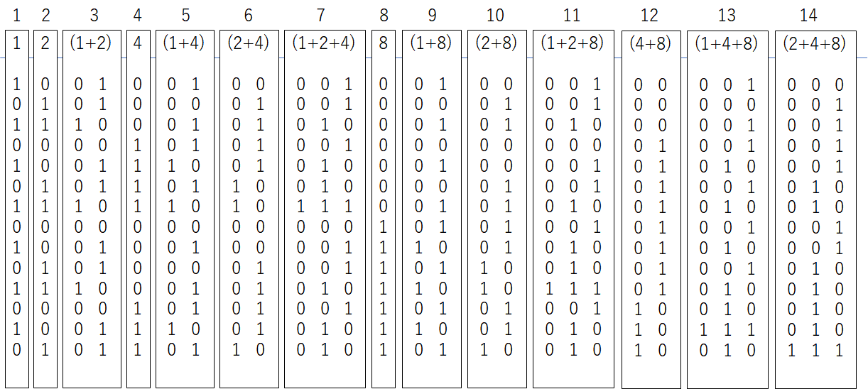
下記は28bitあたり14回のチェックで同定する手法を確認したものである。
連立方程式は$x_{1}~x_{28}$の要素がそれぞれ1か0であることを示す$x_{1}*x_{1}-x_{1}=0$、$x_{2}*x_{2}-x_{2}=0$…$x_{28}*x_{28}-x_{28}=0$の28個の方程式と14回のチェック結果$x_{1}+x_{4}+x_{7}+...=result_{1}$、$=~result_{14}$の計42の方程式を立てこれを解くことで求めたい。
以下のプログラムでは最適な効率かどうかは別にして、bit全探索ではメモリが足りなくなる領域でも答えを求める事が出来ている。
import numpy as np
from sympy import *

def bit2(a,b):
    r = np.array([0,0])
    if (a,b)==(1,0) or (a,b)==(0,1):
        r = np.array([0,1])
    if (a,b)==(1,1):
        r = np.array([1,0])
    return r

def bit3(a,b,c):
    r = np.array([0,0,0])
    if (a,b,c)==(1,0,0) or (a,b,c)==(0,1,0) or (a,b,c)==(0,0,1):
        r = np.array([0,0,1])
    if (a,b,c)==(1,1,0) or (a,b,c)==(0,1,1) or (a,b,c)==(1,0,1):
        r = np.array([0,1,0])
    if (a,b,c)==(1,1,1):
        r = np.array([1,1,1])
    return r

def Solve8(length):
    global iter
    m = 14
    Am = 28
    M = np.zeros((28,14))
    M_list = [[1], [2], [1,2], [4], [1,4], [2,4], [1,2,4], [8], [1,8], [2,8], [1,2,8], [4,8], [1,4,8], [2,4,8]]

    index_list = []
    k = 0
    for i in range(14):
        index_list.append(k)
        k += len(M_list[i])

    k = 0
    for i in range(14):
        index = index_list[i]
        if len(M_list[i])==1:
            for j in range(14):
                M[index,j] = np.array(list(format(j+1, '04b'))).astype('int64')[-1-k]
            k += 1
        if len(M_list[i])==2:
            index2 = index_list[M_list[i][0]-1]
            index3 = index_list[M_list[i][1]-1]
            for j in range(14):
                M[index:index+2,j] = bit2(M[index2,j], M[index3,j])
        if len(M_list[i])==3:
            index2 = index_list[M_list[i][0]-1]
            index3 = index_list[M_list[i][1]-1]
            index4 = index_list[M_list[i][2]-1]
            for j in range(14):
                M[index:index+3,j] = bit3(M[index2,j], M[index3,j], M[index4,j])

    y_check = np.array([1] * int(28))
    x = [Symbol('x%d' % (i)) for i in range(28)]
    result = np.array([0]*14)

    for index in range(0,1008,28):
        y_true2 = y_true[index:index+28]

        eq = []
        for i in range(28):
            eq.append(x[i] * x[i] - x[i])
        for j in range(14):
            result[j] = test(y_check[:np.count_nonzero(M[:,j])], y_true2[M[:,j]==1])
            iter += 1

            eq0 = 0
            for i in range(28):
                if M[i,j]==1:
                    eq0 += M[i,j] * x[i]
            eq.append(eq0 - result[j])
        y_pred[index:index+28] = np.array(solve(eq, x)[0])
---------------------------------------
504 [0 1 1 ... 0 0 0] [0 1 1 ... 0 1 1] 1013
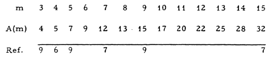
また参考までに$m=16$以降の$A(m)$を見積もると以下の様になる。
$m=63$なら$63/192$及び$27/64$より$N=1024$ならば$63*5+27=342$回となる。この時点で理論上限の$320$にほぼ近い。
ただし、実際の制限として$m=24$あたりから連立方程式を解けなくなる(答えが返ってくるのに非常に時間が掛かる)。また$bit4(a,b,c,d)$に相当する関数が不明である。このため$m=15$以降を一意に解けない。(論文の内容を理解していない)


解9.607回
解3の解き方を思い出してみればチェックするビット数は1024bit→512bit→256bit→…→4bit→2bit→1bitと半分ずつ減らして調べていく。この内、1bitのチェック回数が最も多いのだが、この1bitのチェック自体は効率が悪い。
解2によれば4bitあたり3回で同定できるし、解8によれば28bitあたり14回で同定する方法を示した。
さて、任意長さの1bitずつのチェック回数が$14/28$の割合で済むとき解3のチェック回数はもっと減る。
循環する再帰関数を使っているのでこれの実装は残念ながら容易ではないが(1bitのチェックを先送りして、集めた1bitのチェックが28bitになったら結合した配列のチェックを行い同定し、先送りした場所に結果を戻す)、回数の見積もりだけであるなら1bitチェック回数を$14/28$に換算して計ればよい。
この手法の場合の見積もり回数は平均607回である。
def check2(index, length, upper_result):
    global iter
    result = comit(y_true, index, length)

    if result in [0,length]:
        input_data(y_pred, index, length, result)
        if length==1:                             # 追加
            iter -= 14/28                         # 追加
    else:
        check(index, length//2, result)

    if upper_result is None:
        return

    index += length
    result2 = upper_result - result
    if result2 in [0,length]:
        input_data(y_pred, index, length, result2)
    else:
        check(index, length//2, result2)

def Solve9(length):
    check2(0, 1024, None)
解10.予めの正解率が50%を超えている場合
今回の考え方は初期予測ラベルを全部0として、一部の予測ラベルを1に変えてサブミットを行い、その結果によって予測ラベルを0のままか1に変えるかを決定している。
これは初期予測ラベルを0と1の混ざる配列として、一部の予測ラベルをbit反転を行いサブミットし、その結果によって初期配列からbit反転するか決定するように考えても同じことである。
適応戦略である解9は初期正解率が高い場合、回数を削減する期待値が高くなる。
テストデータが不均衡データか、簡易的なモデルによって予め正解率が$50%$を超えている場合、そのモデルでの予測ラベルを初期予測ラベルとすれば初期予測か、あるいはそれをある範囲でbit反転した結果である可能性は高くなるので、一部の解法(解3、解9)では削減の期待値が大きくなる。一方、解8のような非適応戦略では正解率が非常に高くてもチェック回数は削減されない。
| 2bitで(0,0)か(1,1) | 3bitで(0,0,0)か(1,1,1) | 4bitで(0,0,0,0)か(1,1,1,1) | |
|---|---|---|---|
| 正解率50% | (25+25)/100=0.500 | (125+125)/1000=0.250 | (625+625)/10000=0.1250 |
| 正解率60% | (36+16)/100=0.520 | (216+64)/1000=0.280 | (1296+256)/10000=0.1552 |
| 正解率70% | (49+9)/100=0.580 | (343+27)/1000=0.370 | (2401+81)/10000=0.2482 |
| 正解率80% | (64+4)/100=0.680 | (512+8)/1000=0.520 | (4096+16)/10000=0.4112 |
| 正解率90% | (81+1)/100=0.820 | (729+1)/1000=0.730 | (6561+1)/10000=0.6562 |
| 正解率95% | 0.905 | 0.8575 | 0.8145... |
| 解3 | 解9 | |
|---|---|---|
| 正解率50% | 735 | 607 |
| 正解率60% | 715 | 593 |
| 正解率70% | 655 | 549 |
| 正解率80% | 548 | 465 |
| 正解率90% | 369 | 321 |
| 正解率95% | 232 | 208 |
# y_true = np.random.randint(0, 2, (n))
y_true = np.random.choice(a=[0,1], size=n, p=[0.95,0.05])
正解率が非常に高ければ大きなサブミット回数削減効果が見られる。
$60%$程度の正解率ではサブミットの回数はほとんど削減することは出来ないようでした。
一方$90%$のモデルが公開されているなら$320$回のサブミットでこれを$100%$に出来るでしょう。これは非適応戦略の理論上限の$320$回とほぼ同じです。流石に$100%$出るのは不自然だからと意図的にサブミットを$160$回くらいで止めておけば約$95%$の精度が出ることになります。
K値分類問題
$K$値分類問題に対しても複数の$2$値分類を解くことで求められる。
例えば$N$件の$8$値分類問題を考える。8個のラベルに対してラベル1~4までに1を入れてチェックを行う。この場合、正解ラベルは1~4に含まれているか、いないかの$N$個の$2$値分類問題である。同様にラベル1,2,5,6に1を入れてチェックを行う$2$値分類問題、ラベル1,3,5,7に1を入れてチェックを行う$2$値分類問題を解けばいい。
この$3N$個の$2$値分類問題から$N$個の$8$値分類問題を求めることができる。
また、特定のラベルが問題に対して頻出する偏ったデータでは先に偏ったデータの場所を特定してから残りのラベルを調査した方が回数の削減になる。例えば$N=1024$件の$9$値分類問題で内、$60%$が0ラベルだと知っているなら先に0ラベルの位置を特定すれば、あとは$N=410$の$8$値分類問題となる。
まとめ:
$N=1024$の2値分類問題の場合、$515$回で同定できる手法を示した。
理論的に必要な回数は$N=1024$の場合、$200~320$回なので十分ではないが、解8のmを大きくしていけばその比率に近づくと思われる。
一方、適応戦略の解き方を考えると機械学習で$80%$以上の精度を出せる場合は、適応戦略の解10の方が非適応戦略の解8よりも更に少なくて済む。特に$90%$以上の場合は適応戦略は非適応戦略の理論値よりも良い。
参考: