CMA-ES
前回および前々回に続いてPythonの進化計算ライブラリDeapの紹介の続きをやります。今回はCMA-ESを見ていきます。
まず最初に、CMA-ESがどういったものかを解説したいと思います。CMA-ESは Covariance Matrix Adaptation Evolution Strategy の略で非線形/不連続関数の最適化計算です。簡単に説明すると、探索個体群の生成を多変量正規分布を用いて行い、個体群の評価から多変量正規分布の平均と分散共分散行列を更新させていくという方法です。
今、探索空間が$n$次元で$k$ステップ目の$\lambda(>1)$個の個体群生成を行うとした場合、以下の多変量正規分布から解候補$x_i \in {\bf R}^n(i=1,...,\lambda)$が生成されます。
x_i ~ \sim N(m_k, \sigma_k^2 C_k)
CMA-ESではこの$m_k, \sigma_k^2, C_k$を毎ステップで更新していきます。
Rastrigin関数
今回はRastrigin関数という関数の最適化を行います。Rastrigin関数は最適化アルゴリズムのベンチマーク関数としてよく使われるもので以下の式で表されます。
f(x) = An + \sum_{i=1}^n [ x_i^2 - A\cos(2\pi x_i ) ]
ここで$A=10, x_i \in [-5.12, 5.12]$で、最小になる点が$x=0$で$f(x)=0$です。
matplotlibを使ってちょっと描画してみますと…
from mpl_toolkits.mplot3d import Axes3D
from matplotlib import cm
import matplotlib.pyplot as plt

from deap import benchmarks
import numpy as np

fig = plt.figure()
ax = fig.gca(projection='3d')
X = np.arange(-5.12, 5.12, 0.1)
Y = np.arange(-5.12, 5.12, 0.1)
X, Y = np.meshgrid(X, Y)
Z = [[benchmarks.rastrigin((x, y))[0] for x, y in zip(xx, yy)] for xx, yy in zip(X, Y)]
surf = ax.plot_surface(X, Y, Z, rstride=1, cstride=1, cmap=cm.coolwarm, linewidth=0, antialiased=False)
plt.show()
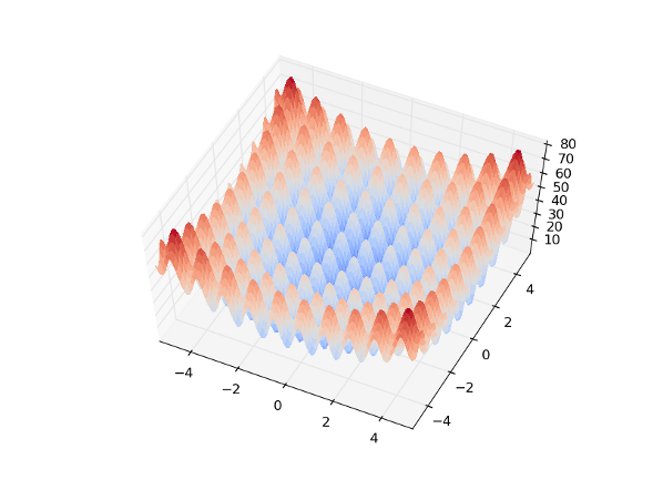
こんな感じでなみなみした関数が出てきます。
サンプルコード
CMA-ESの途中過程でどのような分散共分散行列が生成されるかを確認するために毎ステップでの分散共分散行列を描画するようにしています。
# -*- coding: utf-8 -*-
import numpy

from deap import algorithms
from deap import base
from deap import benchmarks
from deap import cma
from deap import creator
from deap import tools

import matplotlib.pyplot as plt

N = 2  # 問題の次元
NGEN = 50  # 総ステップ数

creator.create("FitnessMin", base.Fitness, weights=(-1.0,))
creator.create("Individual", list, fitness=creator.FitnessMin)

toolbox = base.Toolbox()
toolbox.register("evaluate", benchmarks.rastrigin)

def main():
    numpy.random.seed(64)

    # The CMA-ES algorithm
    strategy = cma.Strategy(centroid=[5.0]*N, sigma=3.0, lambda_=20*N)
    toolbox.register("generate", strategy.generate, creator.Individual)
    toolbox.register("update", strategy.update)

    halloffame = tools.HallOfFame(1)

    halloffame_array = []
    C_array = []
    centroid_array = []
    for gen in range(NGEN):
        # 新たな世代の個体群を生成
        population = toolbox.generate()
        # 個体群の評価
        fitnesses = toolbox.map(toolbox.evaluate, population)
        for ind, fit in zip(population, fitnesses):
            ind.fitness.values = fit

        # 個体群の評価から次世代の計算のためのパラメタ更新
        toolbox.update(population)

        # hall-of-fameの更新
        halloffame.update(population)

        halloffame_array.append(halloffame[0])
        C_array.append(strategy.C)
        centroid_array.append(strategy.centroid)

    # 計算結果を描画
    import matplotlib.pyplot as plt
    import matplotlib.cm as cm
    from matplotlib.patches import Ellipse
    plt.ion()
    fig = plt.figure()
    ax = fig.add_subplot(111)
    X = numpy.arange(-5.12, 5.12, 0.1)
    Y = numpy.arange(-5.12, 5.12, 0.1)
    X, Y = numpy.meshgrid(X, Y)
    Z = [[benchmarks.rastrigin((x, y))[0] for x, y in zip(xx, yy)]
         for xx, yy in zip(X, Y)]
    ax.imshow(Z, cmap=cm.jet, extent=[-5.12, 5.12, -5.12, 5.12])
    for x, sigma, xmean in zip(halloffame_array, C_array, centroid_array):
        # 多変量分布の分散を楕円で描画
        Darray, Bmat = numpy.linalg.eigh(sigma)
        ax.add_artist(Ellipse((xmean[0], xmean[1]),
                              numpy.sqrt(Darray[0]),
                              numpy.sqrt(Darray[1]),
                              numpy.arctan2(Bmat[1, 0], Bmat[0, 0]) * 180 / numpy.pi,
                              color="g",
                              alpha=0.7))
        ax.plot([x[0]], [x[1]], c='r', marker='o')
        ax.axis([-5.12, 5.12, -5.12, 5.12])
        plt.draw()
    plt.show(block=True)

if __name__ == "__main__":
    main()
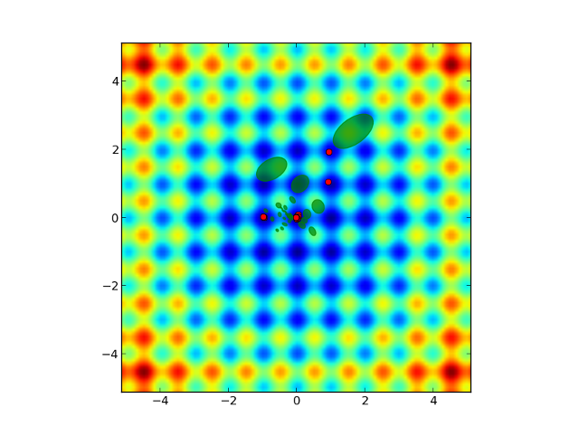
緑の楕円が各ステップの分散共分散行列を表していて、最適解$[0,0]$に近づくにつれて楕円が小さくなって探索範囲が狭くなってきているのが分かります。実際に上のスクリプトを実行するとアニメーション的に新たなステップでの楕円が足されて描画されていくので、楕円の変化がより分かりやすいかと思います。赤の点は各ステップの最も良い解を表していてこちらも最終的に$[0,0]$に集まっています。
参考
CMA-ESのExample:http://deap.gel.ulaval.ca/doc/default/examples/cmaes_plotting.html