More than 5 years have passed since last update.

［翻訳］tidytext vignette: tidytext入門

Posted at 2017-01-22

この文書は，Julia Silge と David Robinson によるRパッケージ tidytext (version 0.1.2) のビネット "Introduction to tidytext" の日本語訳です．

License: MIT

人生がときめくテキスト整然化の魔法

整然データの原則（tidy data principles）¹を用いると，多くのテキストマイニングのタスクをより容易で効果的に，かつ既に広く利用されているツールと整合的なやり方でこなすことができます．整然データフレームを用いてテキストマイニングを行うための基盤は，dplyrやbroom， tidyrやggplot2といったパッケージの中に既に存在しています．このパッケージでは，テキストと整然形式とを相互に変換したり，整然ツールと既存のテキストマイニングパッケージをシームレスに行き来したりすることを可能にするための関数や補助的なデータセットを提供します．

まずは整然テキストマイニングの例をいくつか

ジェーン・オースティンの小説をとても整然としたものにできます！janeaustenrパッケージに収められた，ジェーン・オースティンの完結し出版された小説六編を使って，それらを整然形式に変換しましょう．janeaustenrはこれらの小説を，小説の一行をデータフレームの一行とする形式で提供しています．

library(janeaustenr)
library(dplyr)
library(stringr)

original_books <- austen_books() %>%
  group_by(book) %>%
  mutate(linenumber = row_number(),
         chapter = cumsum(str_detect(text, regex("^chapter [\\divxlc]",
                                                 ignore_case = TRUE)))) %>%
  ungroup()

original_books

## # A tibble: 73,422 × 4
##                     text                book linenumber chapter
##                    <chr>              <fctr>      <int>   <int>
## 1  SENSE AND SENSIBILITY Sense & Sensibility          1       0
## 2                        Sense & Sensibility          2       0
## 3         by Jane Austen Sense & Sensibility          3       0
## 4                        Sense & Sensibility          4       0
## 5                 (1811) Sense & Sensibility          5       0
## 6                        Sense & Sensibility          6       0
## 7                        Sense & Sensibility          7       0
## 8                        Sense & Sensibility          8       0
## 9                        Sense & Sensibility          9       0
## 10             CHAPTER 1 Sense & Sensibility         10       1
## # ... with 73,412 more rows

これを整然データセットとして取り扱うためには，1行1トークンの形式に再構成する必要があります．テキスト列を持つデータフレームを1行1トークン形式に変換するのがunnest_tokens関数です．

library(tidytext)
tidy_books <- original_books %>%
  unnest_tokens(word, text)

tidy_books

## # A tibble: 725,054 × 4
##                   book linenumber chapter        word
##                 <fctr>      <int>   <int>       <chr>
## 1  Sense & Sensibility          1       0       sense
## 2  Sense & Sensibility          1       0         and
## 3  Sense & Sensibility          1       0 sensibility
## 4  Sense & Sensibility          3       0          by
## 5  Sense & Sensibility          3       0        jane
## 6  Sense & Sensibility          3       0      austen
## 7  Sense & Sensibility          5       0        1811
## 8  Sense & Sensibility         10       1     chapter
## 9  Sense & Sensibility         10       1           1
## 10 Sense & Sensibility         13       1         the
## # ... with 725,044 more rows

この関数はtokenizersパッケージを使って各行を単語に分割します．デフォルトではトークン化は語単位で行われますが，他のオプションとして，文字・Nグラム・文・行・段落を単位としたり，正規表現のパターンで区切ったりするものもあります．

さて，データが一行一語形式になったので，これをdplyrのような整然ツールによって操作することができます．anti_joinを用いれば，ストップワード（tidytextのstop_wordsデータセットに入っています）を除去することができます．

data("stop_words")
cleaned_books <- tidy_books %>%
  anti_join(stop_words)

また，countを使って，すべての本を合わせた全体の中で最も出現頻度の高い単語を見つけることもできます．

cleaned_books %>%
  count(word, sort = TRUE)

## # A tibble: 13,914 × 2
##      word     n
##     <chr> <int>
## 1    miss  1855
## 2    time  1337
## 3   fanny   862
## 4    dear   822
## 5    lady   817
## 6     sir   806
## 7     day   797
## 8    emma   787
## 9  sister   727
## 10  house   699
## # ... with 13,904 more rows

感情分析は内部結合（inner join）として実行できます．tidytextパッケージのsentimentsデータセットには，三つの感情語辞書が収められています．NRC辞書で喜び（joy）のスコアが割当てられている単語を見てみましょう．「エマ（Emma）」で最も出現頻度の高い喜びの単語は何でしょうか．

nrcjoy <- get_sentiments("nrc") %>%
  filter(sentiment == "joy")

tidy_books %>%
  filter(book == "Emma") %>%
  semi_join(nrcjoy) %>%
  count(word, sort = TRUE)

## # A tibble: 303 × 2
##       word     n
##      <chr> <int>
## 1     good   359
## 2    young   192
## 3   friend   166
## 4     hope   143
## 5    happy   125
## 6     love   117
## 7     deal    92
## 8    found    92
## 9  present    89
## 10    kind    82
## # ... with 293 more rows

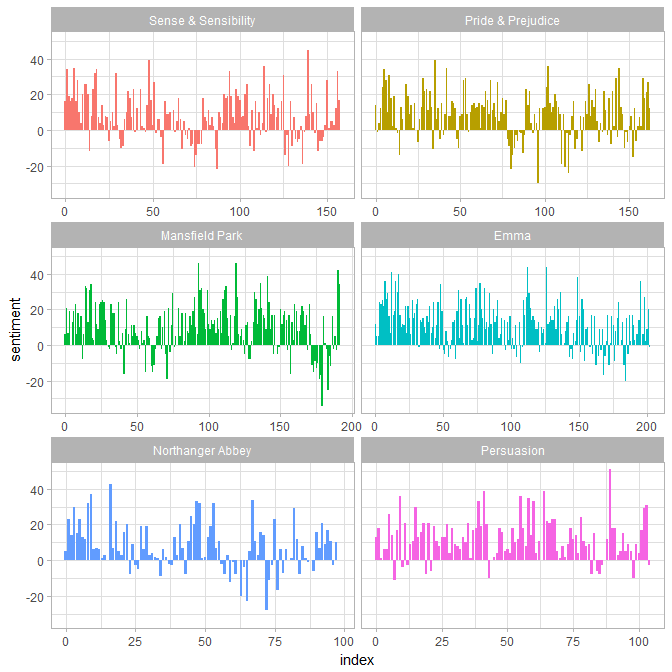
あるいは，各小説の中で感情がどう変化してゆくのかを調べることもできるでしょう．bing辞書を使って各単語の感情スコアを調べて，それから，各小説で定義されたセクションの中のポジティブな単語とネガティブな単語の数を数えてみましょう．

library(tidyr)
bing <- get_sentiments("bing")

janeaustensentiment <- tidy_books %>%
  inner_join(bing) %>%
  count(book, index = linenumber %/% 80, sentiment) %>%
  spread(sentiment, n, fill = 0) %>%
  mutate(sentiment = positive - negative)

こうして，各小説の筋書きに沿って感情スコアをプロットすることができます．

library(ggplot2)

ggplot(janeaustensentiment, aes(index, sentiment, fill = book)) +
  geom_bar(stat = "identity", show.legend = FALSE) +
  facet_wrap(~book, ncol = 2, scales = "free_x")

最も出現頻度の高いポジティブ単語とネガティブ単語

感情と単語が両方入ったデータフレームを持つことの利点は，それぞれの感情に寄与している単語の出現回数を分析できることです．

bing_word_counts <- tidy_books %>%
  inner_join(bing) %>%
  count(word, sentiment, sort = TRUE) %>%
  ungroup()

bing_word_counts

## # A tibble: 2,585 × 3
##        word sentiment     n
##       <chr>     <chr> <int>
## 1      miss  negative  1855
## 2      well  positive  1523
## 3      good  positive  1380
## 4     great  positive   981
## 5      like  positive   725
## 6    better  positive   639
## 7    enough  positive   613
## 8     happy  positive   534
## 9      love  positive   495
## 10 pleasure  positive   462
## # ... with 2,575 more rows

これは視覚的に示すことができます．われわれは整然データフレームを扱うために作られたツールを首尾一貫して使用しているので，ggplot2までパイプを直接つないでいくことができます．

bing_word_counts %>%
  filter(n > 150) %>%
  mutate(n = ifelse(sentiment == "negative", -n, n)) %>%
  mutate(word = reorder(word, n)) %>%
  ggplot(aes(word, n, fill = sentiment)) +
  geom_bar(stat = "identity") +
  theme(axis.text.x = element_text(angle = 90, hjust = 1)) +
  ylab("Contribution to sentiment")

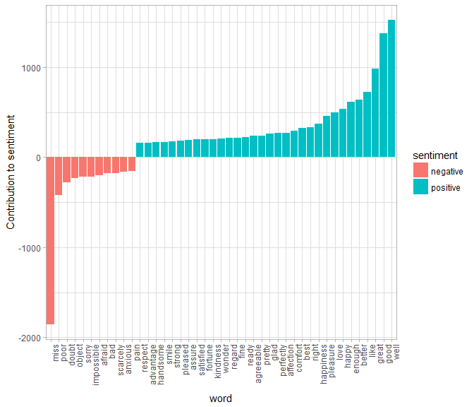
こうすると，この感情分析における変則的な例が見つかります．「miss」という単語がネガティブなものとしてコーディングされていますが，この単語は，ジェーン・オースティンの作品では若い未婚の女性に対する敬称として使われているのです．もしわれわれの目的にとって適切であれば，bind_rowsを使って「miss」をカスタムしたストップワードリストに簡単に加えることができます．

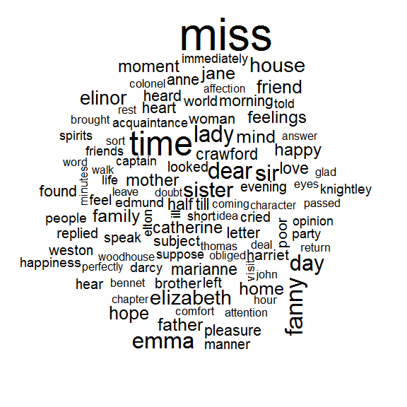
ワードクラウド

整然テキストマイニングの方法が，gpplot2と組み合わせるとうまくいくのを見てきました．しかしデータを整然形式で持っておくのは，他の作図においても同じように有用です．

例としてwordcloudパッケージを考えます．ジェーン・オースティンの作品全体で最も出現頻度の高い単語を再び見てみましょう．

library(wordcloud)

cleaned_books %>%
  count(word) %>%
  with(wordcloud(word, n, max.words = 100))

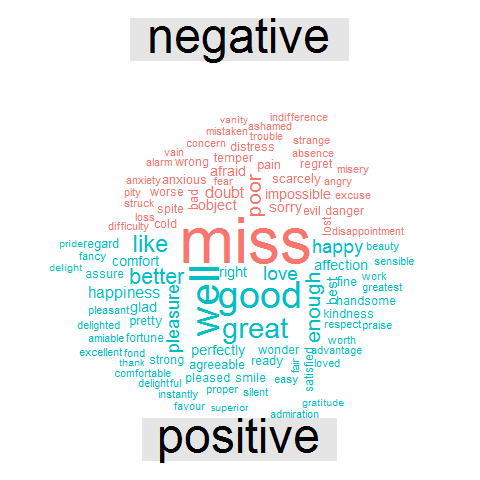
comparison.cloudのような他の関数では，reshape2のacastでデータを行列に変換する必要があるかもしれません．内部結合を用いてポジティブな単語とネガティブな単語にタグ付けし，それから最も出現頻度の高いポジティブな単語とネガティブな単語を見つける感情分析を行ってみましょう．データが整然形式になっているので，データをcomparison.cloudに送る段階までは，すべて結合・パイプとdplyrによって実行できます．

library(reshape2)

tidy_books %>%
  inner_join(bing) %>%
  count(word, sentiment, sort = TRUE) %>%
  acast(word ~ sentiment, value.var = "n", fill = 0) %>%
  comparison.cloud(colors = c("#F8766D", "#00BFC4"),
                   max.words = 100)

単語より長い単位を見る

単語レベルのトークン化によって，多くの役立つ仕事ができますが，時にはテキストを異なった単位で見ることが有用だったり必要だったりすることもあります．たとえば，感情分析アルゴリズムの中には，ユニグラム（単語）を見るだけでなく，文全体の感情を理解しようとするものがあります．こういったアルゴリズムは

I am not having a good day. （私はよい一日を過ごしていない．）

という文が，否定が入っているために，喜びではなくて悲しみを表していることを理解しようとします．Stanford CoreNLPのツールやsentimentr R パッケージ（今のところCRANにはないですがGithubで利用可能です）は，そのような感情分析アルゴリズムの例です．これらを使うために，テキストを文単位にトークン化したくなることがあるかもしれません．

PandP_sentences <- data_frame(text = prideprejudice) %>% 
  unnest_tokens(sentence, text, token = "sentences")

一文だけ見てみましょう．

PandP_sentences$sentence[2]

## [1] "however little known the feelings or views of such a man may be on his first entering a neighbourhood, this truth is so well fixed in the minds of the surrounding families, that he is considered the rightful property of some one or other of their daughters."

エンコーディングがUTF-8のテキストでは，文単位のトークン化に少々問題があるようです．特に対話のセクションで問題があるようです．ASCIIの句読点ではもっとうまくいきます．

unnest_tokensのもう一つのオプションとして，正規表現のパターンを用いてトークンに分割するというものがあります．これを使って，たとえばジェーン・オースティンの小説のテキストを，章ごとに分割したデータフレームにすることができるでしょう．

austen_chapters <- austen_books() %>%
  group_by(book) %>%
  unnest_tokens(chapter, text, token = "regex", pattern = "Chapter|CHAPTER [\\dIVXLC]") %>%
  ungroup()

austen_chapters %>% 
  group_by(book) %>% 
  summarise(chapters = n())

## # A tibble: 6 × 2
##                  book chapters
##                <fctr>    <int>
## 1 Sense & Sensibility       51
## 2   Pride & Prejudice       62
## 3      Mansfield Park       49
## 4                Emma       56
## 5    Northanger Abbey       32
## 6          Persuasion       25

各小説の章の数が正しく再現されました（小説の題名を含む「余分な」一行が付いていますが）．このデータフレームでは，各行が各章に対応しています．

このビネットの最初の方で，一行一語形式に整理した整然データフレームに対して，オースティンの小説の章を特定するために似たような正規表現を使いました．整然テキスト分析を使って，ジェーン・オースティンの各小説において最もネガティブな章はどれか，といった疑問に答えることができます．まず，Bing辞書からネガティブな単語のリストを取得します．次に，章の長さで正規化ができるように，各章の単語数を持つデータフレームを作ります．それから，各章のネガティブな単語の数を特定して，章の全単語数で割ります．ネガティブな単語の割合が最も高いのはどの章でしょうか．

bingnegative <- get_sentiments("bing") %>%
  filter(sentiment == "negative")

wordcounts <- tidy_books %>%
  group_by(book, chapter) %>%
  summarize(words = n())

tidy_books %>%
    semi_join(bingnegative) %>%
  group_by(book, chapter) %>%
  summarize(negativewords = n()) %>%
  left_join(wordcounts, by = c("book", "chapter")) %>%
  mutate(ratio = negativewords/words) %>%
  filter(chapter != 0) %>%
  top_n(1)

## Source: local data frame [6 x 5]
## Groups: book [6]
## 
##                  book chapter negativewords words      ratio
##                <fctr>   <int>         <int> <int>      <dbl>
## 1 Sense & Sensibility      43           161  3405 0.04728341
## 2   Pride & Prejudice      34           111  2104 0.05275665
## 3      Mansfield Park      46           173  3685 0.04694708
## 4                Emma      15           151  3340 0.04520958
## 5    Northanger Abbey      21           149  2982 0.04996647
## 6          Persuasion       4            62  1807 0.03431101

これが，それぞれの本において，章の単語数で正規化したときに最もネガティブな単語が多い章です．これらの章では何が起こっているのでしょうか．「分別と多感（Sense and Sensibility）」の43章では，マリアンが深刻な病気で瀕死となっており，「高慢と偏見（Pride and Prejudice」の34章は，ダーシー氏が最初の（ひどい）求婚を行うところです．「マンスフィールド・パーク（Mansfield Park）」の46章はほとんど終わりに近く，ヘンリーの恥ずべき不貞が発覚するところで，「エマ（Emma」の15章は恐ろしいエルトン氏が求婚するところです．「ノーサンガー・アビー（Northanger Abbey）」の21章ではキャサリンがゴシック小説の殺人の空想にふけったりしています．「説得（Persuation）」の4章は，アンがウェントワース大佐を拒否してどんなに悲しく，ひどい誤りを犯したかを悟る一部始終の回想シーンを読者が読むところです．

原文のリンク先はここ．本文のリンク先は西原史暁氏による翻訳． ↩

You get articles that match your needs
You can efficiently read back useful information
You can use dark theme

What you can do with signing up