Visualising intersection-over-union relationship via Venn Diagrams

In my work, I sometimes have to explain how certain datasets changed over time. For example, recently I had to crawl the portion of OSM dataset containing the data related to Japan, and upload it to BigQuery. The last time this task was done in our company, was around three years ago, and by a different method. So, naturally, the resulting set turned out to be a bit different, with some roads present only in recently created dataset, some present only in original dataset, and some present in both.

I therefore, had to present the percentage of data in each of these categories, so my superior could decide whether the change should be considered big or not.

Now, the way I do it normally, is just by giving percentages, e.g.
1. 15% of roads are contained in new dataset, but not in old
1. 9% are contained in old, but not in new
1. 75% are contained in both.

However, I have noticed myself that laid out raw numbers are sometimes difficult to process and imagine. For example, "75%" -- is it big or small change? And which set is bigger, after all, the new one, or the old one?

I figured out that it would be nice to somehow visualize the relationship between those two sets. Now, it occured to me that Venn diagrams would be a great way to do so, with its simple apparent structure (all images created with draw.io):

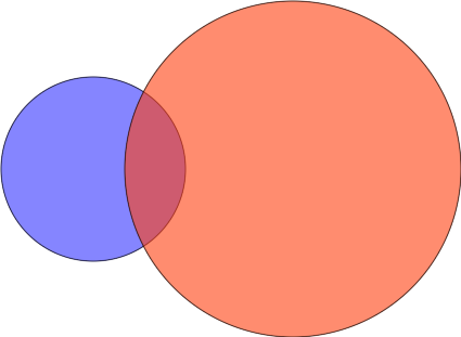
It therefore would only remain to compute the radii of circles and the distance between their centers, so that intersection and set differences would give the required fractions. More precisely, suppose we are given three positive numbers $a,b,c$ which sum up to one:

$$ a+b+c=1; a,b,c>0$$

Now, suppose they denote the fractions of area of union of two circles, corresponding to
1. part of left circle (shaded in blue), which lies outside right circle (shaded in red);
1. intersection of two circles;
1. part of right circle, which lies outside left circle;

as shown on diagram:

And what we want to compute (i.e. express through $a,b,c$), are the
1. radius $R$ of left (red) circle;
1. radius $r$ of right (blue) circle;
1. distance $x$ between centers of circles (we assume that circles lie on horizontal line).

One fact to mention, is that one can easily convince oneself that by multiplying/dividing all three numbers $R,r,x$ by the same multiplier, corresponding fractions $a,b,c$ do not change, hence the numbers $R,r,x$ are only defined up to a common multiple. Therefore, we can safely assume that $r=1$ and only solve for $r,x$.

Now, the great Circle-Circle Intersection article at Wolfram provides us with necessary formulae to compute $a,b,c$ in terms of $R,r,x$, thus giving us the inverse transform to what we need:

$$
a*(\pi R^2 + \pi r^2 - A) = \pi R^2-A
$$

$$
b*(\pi R^2 + \pi r^2 - A) = A
$$

$$
c*(\pi R^2 + \pi r^2 - A) = \pi r^2 - A,
$$

where $A$ denotes the area of circle intersection and is given via

$$
A = A(R,r,d) = r^2 \cos^{-1} \left(\frac{d^2+r^2-R^2}{2dr}\right)+
R^2 \cos^{-1} \left(\frac{d^2+R^2-r^2}{2dR}\right) -
\frac{1}{2}\sqrt{(-d+r+R)(d+r-R)(d-r+R)(d+r+R)}
$$

Then, we only need to solve this. First, let us solve for $r$:

$$
\frac{\pi r^2}{\pi R^2} = \frac{b+c}{a+b} \implies r=R\sqrt{\frac{b+c}{a+b}} = \sqrt{\frac{b+c}{a+b}}.
$$

Unfortunately, solving for $d$ has proven to be considerably more formiddable task (due to the complexity of expression for $A$), and I was unable to derive an explicit formula. So we will resort to numerical methods.

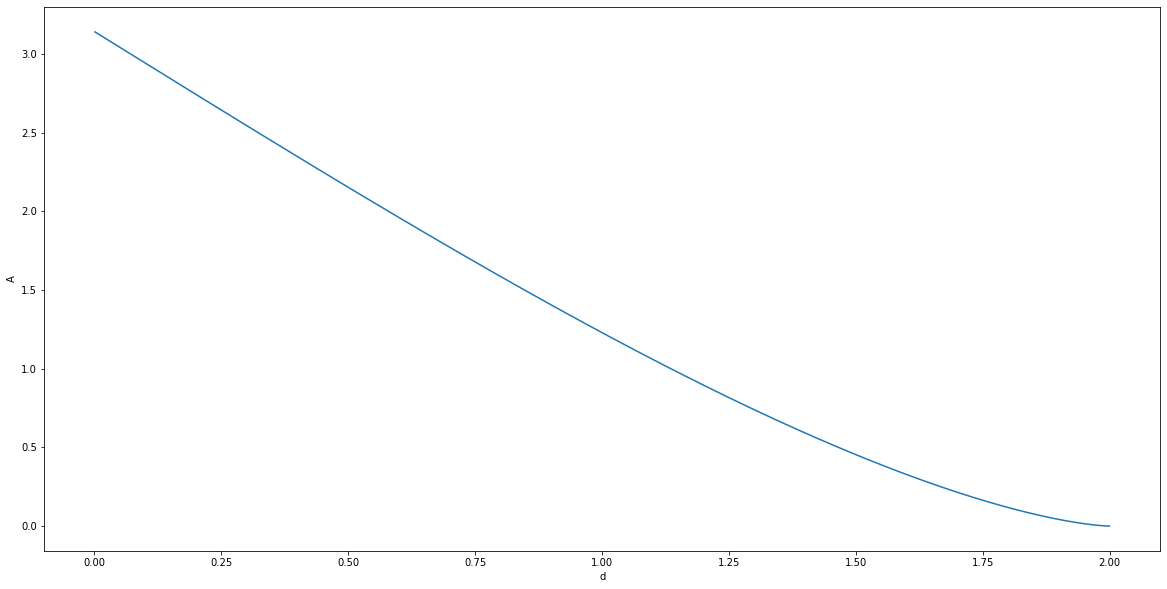
Now, one thing to notice, is that with $R,r$ fixed, $A$ is a decreasing function of $d$. In order to convince yourself of this (convince, but not to prove!), run the following code cell several times.

import pandas as pd
import numpy as np
import seaborn as sns
import matplotlib.pyplot as plt

def A(r,R,d):
    _A = r**2* np.arccos((d**2+r**2-R**2)/(2*d*r)) + R**2* np.arccos((d**2+R**2-r**2)/(2*d*R))-1/2*np.sqrt((-d+r+R)*(d+r-R)*(d-r+R)*(d+r+R))
    return _A

# r,R = 1,np.abs(np.random.randn(1)+1)[0]
r,R = 1,np.abs((np.random.randn()*0.001+1))
print((r,R))
plt.subplots(figsize=(20,10))
_STEP = 1e-3
sns.lineplot(
    data=pd.DataFrame([
        {
            "d":d,
            "A":A(r,R,d),
            "a":(-d+r+R)*(d+r-R)*(d-r+R)*(d+r+R)/d**2,
        }
        for d
        in np.arange(np.abs(r-R)+_STEP,r+R-_STEP,_STEP)
    ]),
    x="d",
    y="A",
#     y="a",
)

Hopefully, now that you are a believer, let me explain, why this is important. The monotonicity allows us to use bisection to solve inverse problem instead of a simple grid search. Note that this is critical, as bisection is asymptotically more efficient than grid search: while the latter has to take linear number of steps to achieve given accuracy, the former requires only logarithmic.

Now, the formal proof of the fact that $A$ is decreasing as a function of $d$ is somewhat lengthy and is given in appendix (see at the end of an article).

All of this lengthy theory was necessary to write the following function:

import numpy as np


def _A(R,r,d):
    return r**2*np.arccos((d**2+r**2-R**2)/(2*d*r))+R**2*np.arccos(
        (d**2+R**2-r**2)/(2*d*R)) - 1/2*np.sqrt((-d+r+R)*(d+r-R)*(d-r+R)*(d+r+R))


def solve_d_r(a, b, c=None, R=1, return_debug_info=False,tol=1e-9):
    """
    return d,r

    formula for two circles' intersection area and notation taken from https://mathworld.wolfram.com/Circle-CircleIntersection.html
    """
    if c is None:
        assert a>0 and b>0 and a+b<1
        c = 1-a-b
    else:
        assert a > 0 and b > 0 and c > 0
        a, b, c = [x/np.sum([a, b, c]) for x in [a, b, c]]

    r = R*np.sqrt((b+c)/(a+b))
    target_A = b*(np.pi*R**2+np.pi*r**2)/(1+b)

    le,ri = np.abs(r-R),R+r
    while ri-le>tol:
        m = (le+ri)/2
        A = _A(R,r,m)
        if A<target_A:
            ri=m
        else:
            le=m
    return (le+ri)/2,r

The sample call would be

b,a = 3/5,1/10
d,r = solve_d_r(
    b=b,
    a=a,
)
d,r

(0.3999826353680148, 1.1338934190276817)

We then can draw the Venn diagram via the following code

import matplotlib.pyplot as plt

fig, ax = plt.subplots(figsize=(10,10)) # note we must use plt.subplots, not plt.subplot
plt.axis('off')
R = 0.3
alpha = 0.2
ax.add_patch(plt.Circle((0.5, 0.5), R, color="blue",alpha=alpha))
ax.add_patch(plt.Circle((0.5+d*R, 0.5), r*R, color="red",alpha=alpha))

ax

Further work

1. the algorithm presented can be easily generalized to draw the Venn diagrams corresponding to relation between the three sets, not two, e.g.

(the image is taken from Wikipedia)

Appendix: proof of the fact that $A$ is decreasing with $d$

First, freshman Calculus suggests us to take a partial derivative of $A(R,r,d)$ with respect to $d$:

import sympy
R,r,x,d = [sympy.Symbol(x) for x in "Rrxd"]

A = r**2* sympy.acos((d**2+r**2-R**2)/(2*d*r)) + R**2* sympy.acos((d**2+R**2-r**2)/(2*d*R))-1/2*sympy.sqrt((-d+r+R)*(d+r-R)*(d-r+R)*(d+r+R))
expr1 = sympy.simplify(
    sympy.diff(A,d),
    rational=True,
    positive=True,
    inverse=True,
)
expr1

$\displaystyle \frac{R \sqrt{\frac{4 d^{2} r^{2} - \left(- R^{2} + d^{2} + r^{2}\right)^{2}}{d^{2} r^{2}}} \left(- R + d + r\right) \left(R - d + r\right) \left(R + d - r\right) \left(R + d + r\right) \left(R^{2} - d^{2} - r^{2}\right) + \frac{d^{2} \sqrt{\frac{4 R^{2} d^{2} - \left(R^{2} + d^{2} - r^{2}\right)^{2}}{R^{2} d^{2}}} \sqrt{\frac{4 d^{2} r^{2} - \left(- R^{2} + d^{2} + r^{2}\right)^{2}}{d^{2} r^{2}}} \sqrt{\left(- R + d + r\right) \left(R - d + r\right) \left(R + d - r\right) \left(R + d + r\right)} \left(- \left(- R + d + r\right) \left(R - d + r\right) \left(R + d - r\right) - \left(- R + d + r\right) \left(R - d + r\right) \left(R + d + r\right) + \left(- R + d + r\right) \left(R + d - r\right) \left(R + d + r\right) - \left(R - d + r\right) \left(R + d - r\right) \left(R + d + r\right)\right)}{4} + r \sqrt{\frac{4 R^{2} d^{2} - \left(R^{2} + d^{2} - r^{2}\right)^{2}}{R^{2} d^{2}}} \left(- R + d + r\right) \left(R - d + r\right) \left(R + d - r\right) \left(R + d + r\right) \left(- R^{2} - d^{2} + r^{2}\right)}{d^{2} \sqrt{\frac{4 R^{2} d^{2} - \left(R^{2} + d^{2} - r^{2}\right)^{2}}{R^{2} d^{2}}} \sqrt{\frac{4 d^{2} r^{2} - \left(- R^{2} + d^{2} + r^{2}\right)^{2}}{d^{2} r^{2}}} \left(- R + d + r\right) \left(R - d + r\right) \left(R + d - r\right) \left(R + d + r\right)}$

This expression is a product

expr1.func

sympy.core.mul.Mul

with the following multiplicands

from IPython.display import display
for i,arg in enumerate(expr1.args):
    print(f"#{i} => ")
    display(arg)

#0 => 

$\displaystyle \frac{1}{d^{2}}$

#1 => 

$\displaystyle \frac{1}{\sqrt{\frac{4 R^{2} d^{2} - \left(R^{2} + d^{2} - r^{2}\right)^{2}}{R^{2} d^{2}}}}$

#2 => 

$\displaystyle \frac{1}{\sqrt{\frac{4 d^{2} r^{2} - \left(- R^{2} + d^{2} + r^{2}\right)^{2}}{d^{2} r^{2}}}}$

#3 => 

$\displaystyle \frac{1}{R + d + r}$

#4 => 

$\displaystyle \frac{1}{R + d - r}$

#5 => 

$\displaystyle \frac{1}{R - d + r}$

#6 => 

$\displaystyle \frac{1}{- R + d + r}$

#7 => 

$\displaystyle R \sqrt{\frac{4 d^{2} r^{2} - \left(- R^{2} + d^{2} + r^{2}\right)^{2}}{d^{2} r^{2}}} \left(- R + d + r\right) \left(R - d + r\right) \left(R + d - r\right) \left(R + d + r\right) \left(R^{2} - d^{2} - r^{2}\right) + \frac{d^{2} \sqrt{\frac{4 R^{2} d^{2} - \left(R^{2} + d^{2} - r^{2}\right)^{2}}{R^{2} d^{2}}} \sqrt{\frac{4 d^{2} r^{2} - \left(- R^{2} + d^{2} + r^{2}\right)^{2}}{d^{2} r^{2}}} \sqrt{\left(- R + d + r\right) \left(R - d + r\right) \left(R + d - r\right) \left(R + d + r\right)} \left(- \left(- R + d + r\right) \left(R - d + r\right) \left(R + d - r\right) - \left(- R + d + r\right) \left(R - d + r\right) \left(R + d + r\right) + \left(- R + d + r\right) \left(R + d - r\right) \left(R + d + r\right) - \left(R - d + r\right) \left(R + d - r\right) \left(R + d + r\right)\right)}{4} + r \sqrt{\frac{4 R^{2} d^{2} - \left(R^{2} + d^{2} - r^{2}\right)^{2}}{R^{2} d^{2}}} \left(- R + d + r\right) \left(R - d + r\right) \left(R + d - r\right) \left(R + d + r\right) \left(- R^{2} - d^{2} + r^{2}\right)$

Due to triangle inequalities

$$
r\leq d+R, d\leq R+r, R\leq d+r,
$$
we see that all expressions except of the last one (e.g. #7) are non-negative. Hence, it suffices to show that #7 is negative.

Now, we will use a bit of geometry to simplify the expression:
note that the radii $R$, $r$ and the segment connecting circle centers $d$ form a triangle, as shown on the diagram below:

Now, we will call the angles of this triangle lying against segments $R$, $r$ and $d$ as $\alpha,\beta$ and $\delta$ respectively. Then, the law of cosines tells us that

$$
R^2+d^2-r^2 = 2Rd\cos(\beta)
$$

$$
-R^2+d^2+r^2 = 2rd\cos(\alpha)
$$

$$
-R^2+d^2-r^2 = -2Rr\cos(\delta)
$$

which together with the difference of two squares formula
$$ (a-b)(a+b) = a^2-b^2$$
allows to simplify the expression #7 above as

def _rec_apply(expr,s,r=None):
    if r is None:
        r = sympy.simplify(s)
    if sympy.simplify(expr-s)==0:
        return r
    elif expr.func in [sympy.core.add.Add,sympy.core.mul.Mul] :
        return expr.func(*[_rec_apply(arg,s,r) for arg in expr.args])
    else:
        return expr

beta,alpha,delta = [sympy.Symbol(s) for s in "beta,alpha,delta".split(",")]
R,d,r = [sympy.Symbol(k) for k in "Rdr"]
_expr = expr2.subs([
    (R**2+d**2-r**2, 2*R*d*sympy.cos(beta)),
    (-R**2+d**2+r**2,2*r*d*sympy.cos(alpha))
])
_expr = sympy.trigsimp(_expr)
_expr = _rec_apply(
    _expr,
    -(-R + d + r)*(R - d + r)*(R + d - r) - (-R + d + r)*(R - d + r)*(R + d + r) + (-R + d + r)*(R + d - r)*(R + d + r) - (R - d + r)*(R + d - r)*(R + d + r), 
)
_expr = _expr.subs(-R**2+d**2-r**2,-2*R*r*sympy.cos(delta))
_expr = _expr.subs([(sympy.sqrt(sympy.sin(x)**2),sympy.sin(x)) for x in [alpha,beta,delta]])
_expr

_expr = sympy.trigsimp(_expr.subs((-𝑅+𝑑+𝑟)*(𝑅-𝑑+𝑟)*(𝑅+𝑑-𝑟)*(𝑅+𝑑+𝑟), 4*R**2*d**2-4*R**2*d**2*(sympy.cos(beta))**2)).subs(
    sympy.sqrt(R**2*d**2*sympy.sin(beta)**2),
    R*d*sympy.sin(beta),
)
_expr

sympy.factor(_expr)

$\displaystyle - 16 R^{2} d^{3} r \left(R \sin{\left(\alpha \right)} \cos{\left(\alpha \right)} + R \sin{\left(\beta \right)} \cos{\left(\beta \right)} + d \sin{\left(\alpha \right)} \cos{\left(\delta \right)}\right) \sin^{2}{\left(\beta \right)}$

We are in a good shape, as expression is much simpler than before, and we only need to show that it's non-positive. Now, ignoring the obviously non-negative factors, it all reduces to showing the non-negativity of

$$
R\sin(\alpha)\cos(\alpha) + R\sin(\beta)\cos(\beta) + d\sin(\alpha)\cos(\delta)
$$

Now, employing the law of sines we see that
$$
d\sin(\alpha) = R\sin(\delta),
$$
hence it suffices to show the non-negativity of

$$
\sin(\alpha)\cos(\alpha) + \sin(\beta)\cos(\beta) + \sin(\delta)\cos(\delta).
$$

Finally, employing the trigonometric formulae

$$
\sin(x)\cos(x)=\sin(2x)/2
$$
$$
\sin(x)+\sin(y) = 2\sin((x+y)/2)\cos((x-y)/2),
$$

and using the fact that $\delta=\pi-\alpha-\beta$ and hence $\sin(\delta)=\sin(\alpha+\beta)$ and $\cos(\delta)=-\cos(\alpha+\beta)$, we see that we only need to show the non-negativity of

$$
\sin(\alpha+\beta)\cos(\alpha-\beta) - \sin(\alpha+\beta)\cos(\alpha+\beta),
$$

thus it remains to show that $\cos(\alpha-\beta)-\cos(\alpha+\beta)$ is non-negative. But this is easy to see, since employing the formula $\cos(x)-\cos(y)=-2\sin((x+y)/2)\sin((x-y)/2)$ gives

$$
\cos(\alpha-\beta)-\cos(\alpha+\beta) = -2\sin(\alpha)\sin(-\beta)=\sin(\alpha)\sin(\beta)\geq0.
$$