In this note I would like to briefly introduce the possibility of using Kepler.GL in
Jupyter notebooks. To cite the official webpage,
Kepler.gl is a powerful open source geospatial analysis tool for *large-scale* data sets.
Intro: Why use Kepler.GL in Jupyter?
To my knowledge, the standard GeoVisualization solution for use in Jupyter is
folium.
I think that using Kepler.GL instead of folium can not only be interesting for the sake of variety, but also due to following
reasons:
- Kepler.GL is high-performant, i.e. it can load big chunks of geodata and still remain responsive;
- Kepler.GL has rich interface: one can easily add/remove datasets and/or layers so to create rich interactive maps, which
can then be exported to JSON or stand-alone HTML;
Installing Kepler.GL widget
Prerequisites
Note that more detailed instructions
are given at references
- Python 3
- Mac OS (I have tried these intsructions on Mac OS only)
- Homebrew
Installation
pip3 install keplergl
pip3 install ipywidgets
brew install node@10
jupyter labextension install @jupyter-widgets/jupyterlab-manager keplergl-jupyter
jupyter notebook
Displaying the widget
Once you have installed the widget, using it is pretty easy:

As mentioned before, widget is fully interactive. At every point, however, one can dump the widget's internal state as

To load the saved internal state into a freshly-created widget, one can do as follows
w = kepler.KeplerGl()
w.config = config
# or directly at the construction
w = kepler.KeplerGl(config=config)
Note that datasets are not included into config (i.e. they have to be passed at creation).
Loading data into widget
Data Sources
In principle, you can use multiple sources to load data into Kepler.GL widget:
I will concentrate on the latter one. However, for the completeness, here are the
demo notebooks from the official documentation corresponding to first two items:
geojson,
geopandas.
A Few Concepts
Before we begin, a word about terminology. While working with Kepler.GL, one distinguishes
datasets
: which are the chunks of raw
data one wants to analyze (think of them as tables), and
layers
: which are layers of data visualization.
Kepler.GL comes with following layer types out-of-the-box: Point, Arc, Cluster, Line, Grid, Polygon, Icon, Heatmap and Hexbin.
The relationship between datasets and layers is one-to-many, that is one can create several layers from one dataset. The
relationship between two is further guided by
filters
: which allow to have only subset of data being visualized.
In principle, after datasets are added, one has to create layers and filters manually, either by using Kepler.GL's UI interface,
or by interacting with widget through the Python API. However, Kepler.GL is
smart enough
to automatically add layers and filters based on dataset in
some cases.
For simplicity, I will never add layers manually in examples below, relying instead on Kepler.GL's built-ins.
Adding Point layers

Note that Kepler.GL automatically created Point layer and filter for Time.
Adding Arc and Line layers
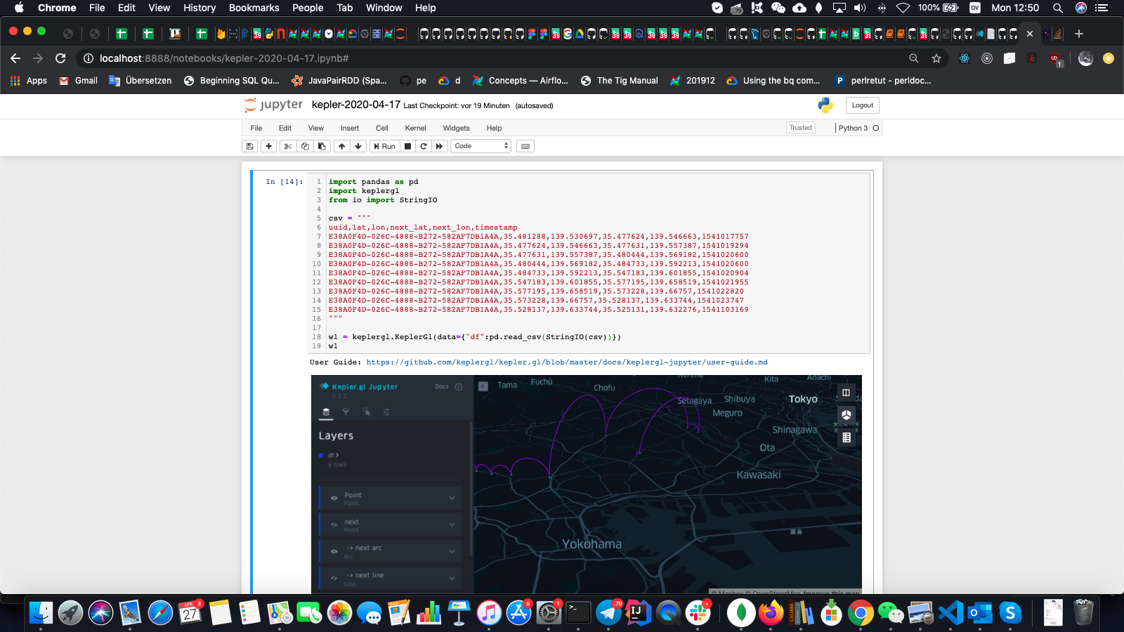
Note that although Arc and Line layers were automatically created, there are hidden by default, so I had to show them
via Kepler.GL's UI.
Adding H3 layer
