回帰分析というと一般的には最小二乗法を用いた線形回帰として
y=ax+b
を想像される方も多いと思いますが、Scikit-Learnでは多項式回帰を行なったり指数関数での回帰(対数回帰)もできます。
今回はその機能を紹介してみようと思います。
多項式回帰
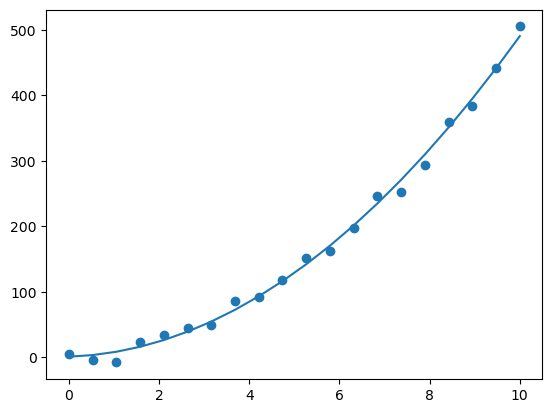
まずは多項式回帰の分かりやすい例として運動エネルギーの回帰をしてみようと思います。
運動エネルギーは公式にすると
K=\frac{1}{2}mv^2
になります。
ではこれについて実際にそれっぽい乱数を観測データとして回帰してみましょう。
プログラム
ノイズは標準偏差10で0を中心としたものとしています。
また、「PolynomialFeatures」を使い多項式にします。
from sklearn.linear_model import LinearRegression as LR
from sklearn.preprocessing import PolynomialFeatures
import numpy as np
import matplotlib.pyplot as plt

v = np.linspace(0, 10, 20).reshape(-1, 1)
m = 10
K = (m * v * v) / 2
K = K + np.random.normal(loc=0, scale=10, size=(len(K), 1))
poly2 = PolynomialFeatures(degree=2)
v_poly = poly2.fit_transform(v)
model = LR()
model.fit(v_poly, K)
y_pred = model.predict(v_poly)
plt.scatter(v, K)
plt.plot(v, y_pred)
plt.show()
print(model.coef_)
print(model.intercept_)
[[0.         2.22676303 4.67129704]]
[0.85771507]
結構ちゃんと回帰できていることが分かります。また、2乗項も質量の半分である5に近い「4.67129704」となっており近似できました。
片対数
データの参考はこちらを参考にしました
プログラム
ライブラリとして「TransformedTargetRegressor」を使います。
from sklearn.compose import TransformedTargetRegressor
from sklearn.linear_model import LinearRegression as LR
import numpy as np
import matplotlib.pyplot as plt
t = np.linspace(0, 100, 11).reshape(-1, 1)
Q = np.array([1.5, 0.91, 0.552, 0.335, 0.203, 0.123, 0.0747, 0.0453, 0.0275, 0.0167, 0.0101])
model = TransformedTargetRegressor(regressor=LR(), func=np.log, inverse_func=np.exp)
model.fit(t, Q)
y_pred = model.predict(t)
plt.scatter(t, Q)
plt.plot(t, y_pred)
plt.grid(which="both")
plt.show()
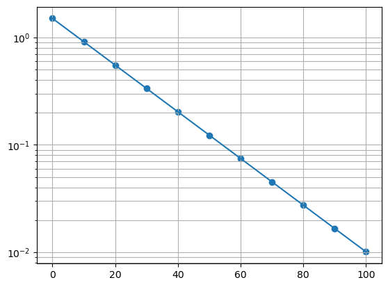
plt.scatter(t, Q)
plt.plot(t, y_pred)
plt.yscale("log")
plt.grid(which="both")
plt.show()
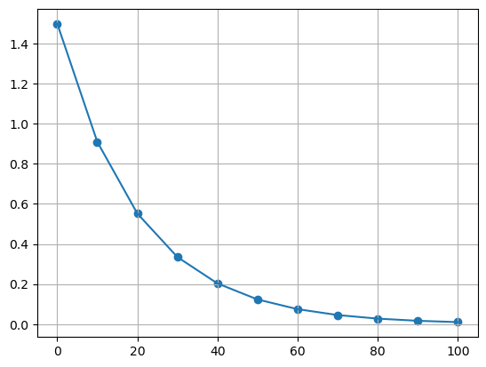

ここから片対数グラフの解釈を行い定式化します。
両対数
from sklearn.linear_model import LinearRegression as LR
from sklearn.compose import TransformedTargetRegressor
from sklearn.preprocessing import FunctionTransformer
import numpy as np
import matplotlib.pyplot as plt
V=np.array([3, 5, 7, 10, 15, 20, 30, 40, 60, 80, 100])
F=np.array([0.4, 1.1, 2.3, 4.5, 9.6, 17, 41, 70, 150, 290, 440])
trans = FunctionTransformer(np.log1p, validate=True)
V_trans = trans.transform(V.reshape(-1, 1))
V_trans = np.array(V_trans)
model = TransformedTargetRegressor(regressor=LR(), func=np.log, inverse_func=np.exp)
model.fit(V_trans, F)
y_pred = model.predict(V_trans)
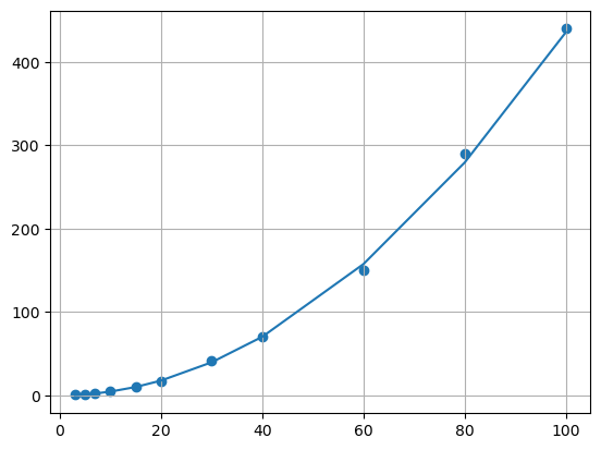
plt.scatter(V, F)
plt.plot(V, y_pred)
plt.grid(which="both")
plt.show()
plt.scatter(V, F)
plt.plot(V, y_pred)
plt.xscale("log")
plt.yscale("log")
plt.grid(which="both")
plt.show()


これで両対数の回帰ができました。最後ズレていますが方法としてはこのようになります。
補足
読者の中で統計2級を持っている方なら分かると思いますが、回帰分析の目的変数や説明変数にlogを用いる事でこんな難しいやり方使わなくても実際には回帰ができます。
片対数
ここでは目的変数のみlogを使います。一度logを使ってモデルを作って回帰し、最後に予測値を自然対数を使います。
from sklearn.linear_model import LinearRegression as LR
import numpy as np
import matplotlib.pyplot as plt

t = np.linspace(0, 100, 11).reshape(-1, 1)
Q = np.array([1.5, 0.91, 0.552, 0.335, 0.203, 0.123, 0.0747, 0.0453, 0.0275, 0.0167, 0.0101])

logQ = np.log(Q)
model = LR()
model.fit(t, logQ)
y_pred = model.predict(t)
plt.scatter(t, Q)
plt.grid(which="both")
plt.plot(t, np.exp(y_pred))
plt.show()
plt.scatter(t, Q)
plt.grid(which="both")
plt.plot(t, np.exp(y_pred))
plt.yscale("log")
plt.show()
print(model.coef_)
print(model.intercept_)

[-0.04999548]
0.4055324342148001
このため回帰式は
Q=e^{-0.04999548t+0.4055324342148001}
となり、これを実際に試してみます。
pred = np.exp(t*model.coef_[0]+model.intercept_)
plt.scatter(t, pred)
plt.grid(which="both")
plt.plot(t, pred)
plt.show()
plt.scatter(t, pred)
plt.grid(which="both")
plt.plot(t, pred)
plt.yscale("log")
plt.show()


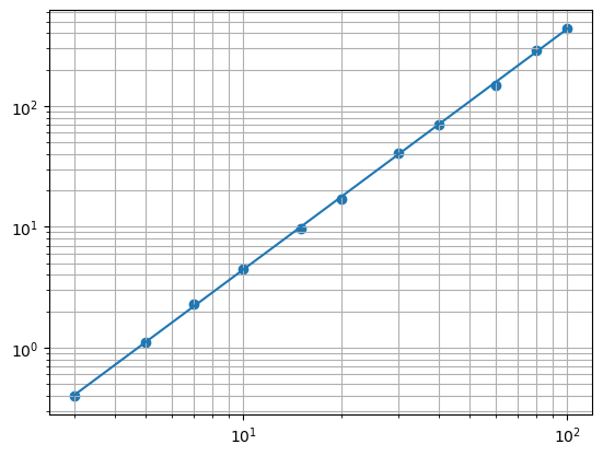
両対数
両対数の場合グラフにする時説明変数であるxだけは元に戻さないでグラフにします。
from sklearn.linear_model import LinearRegression as LR
import numpy as np
import matplotlib.pyplot as plt

V=np.array([3, 5, 7, 10, 15, 20, 30, 40, 60, 80, 100])
F=np.array([0.4, 1.1, 2.3, 4.5, 9.6, 17, 41, 70, 150, 290, 440])

logV = np.log(V).reshape(-1, 1)
logF = np.log(F)
model = LR()
model.fit(logV, logF)
y_pred = model.predict(logV)
plt.scatter(V, F)
plt.plot(V, np.exp(y_pred))
plt.grid(which="both")
plt.show()
plt.scatter(V, F)
plt.plot(V, np.exp(y_pred))
plt.xscale("log")
plt.yscale("log")
plt.grid(which="both")
plt.show()
print(model.coef_)
print(model.intercept_)


[1.99245318]
-3.0977976975026027
さっきは一番最後の値がずれていましたが今度はズレていない事が分かります。
数式にするとこうなります(すみません数学忘れたのでlogを外せてません)
F=e^{1.99245318\ln{V}-3.0977976975026027}
pred = np.exp(model.coef_[0]*np.log(V)+model.intercept_)
plt.scatter(V, F)
plt.plot(V, pred)
plt.grid(which="both")
plt.show()
plt.scatter(V, F)
plt.plot(V, pred)
plt.xscale("log")
plt.yscale("log")
plt.grid(which="both")
plt.show()
2乗項
先ほどの運動エネルギーについても平方根を目的変数に使うと回帰ができます。
ただしこの手法では平方根の性質上必ず目的変数の値が正でないといけません。
from sklearn.linear_model import LinearRegression as LR
import numpy as np
import matplotlib.pyplot as plt

v = np.linspace(0, 10, 20).reshape(-1, 1)
m = 10
K = (m * v * v) / 2
K = abs(K + np.random.normal(loc=0, scale=10, size=(len(K), 1)))
sqrK = abs(np.sqrt(K))
model = LR()
model.fit(v, sqrK)
y_pred = model.predict(v)
plt.scatter(v, K)
plt.plot(v, y_pred**2)
plt.show()

参考文献(というか使ったデータ)
電気基礎実験 <<グラフ処理>>
https://slidesplayer.net/slide/11539427/