ロジスティック回帰はライブラリで違う

データ分析に使うライブラリとして古典的な機械学習がベースのScikit-Learnと数理モデルがベースのstatsmodelsがあります。
重回帰分析をやる分には結果が同じになりますが、ロジスティック回帰だと実は結果が異なるようになります。

決定境界の描画関数

Scikit-Learn用

from sklearn import preprocessing
import matplotlib.pyplot as plt
import numpy as np
def showline_clf(x, y, model, modelname, x0="x0", x1="x1"):
    fig, ax = plt.subplots(figsize=(8, 6))
    X, Y = np.meshgrid(np.linspace(*ax.get_xlim(), 1000), np.linspace(*ax.get_ylim(), 1000))
    XY = np.column_stack([X.ravel(), Y.ravel()])
    x = preprocessing.minmax_scale(x)
    model.fit(x, y)
    Z = model.predict(XY).reshape(X.shape)
    plt.contourf(X, Y, Z, alpha=0.1, cmap="brg")
    plt.scatter(x[:, 0], x[:, 1], c=y, cmap="brg")
    plt.xlim(min(x[:, 0]), max(x[:, 0]))
    plt.ylim(min(x[:, 1]), max(x[:, 1]))
    plt.title(modelname)
    plt.colorbar()
    plt.xlabel(x0)
    plt.ylabel(x1)
    plt.show()

statsmodels用

from sklearn import preprocessing
import matplotlib.pyplot as plt
import numpy as np
def showline_clf2(x, y, model, modelname, x0="x0", x1="x1"):
    fig, ax = plt.subplots(figsize=(8, 6))
    X, Y = np.meshgrid(np.linspace(min(x[:, 1]), max(x[:, 1]), 1000), np.linspace(min(x[:, 2]), max(x[:, 2]), 1000))
    XY = []
    for i in range(len(X.ravel())):
        XY.append([1, X.ravel()[i], Y.ravel()[i]])
    Z = np.argmax(model.predict(XY), axis=1).reshape(X.shape)
    plt.contourf(X, Y, Z, alpha=0.1, cmap="brg")
    plt.scatter(x[:, 1], x[:, 2], c=y, cmap="brg")
    plt.title(modelname)
    plt.colorbar()
    plt.xlabel(x0)
    plt.ylabel(x1)
    plt.show()

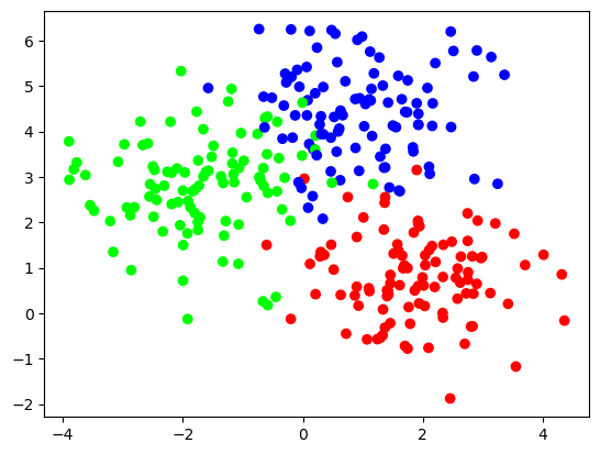
データの読み込み

x, y = make_blobs(n_samples=300, centers=3, random_state=0, cluster_std=1.0)
plt.scatter(x[:, 0], x[:, 1], c=y, cmap="brg")
plt.show()

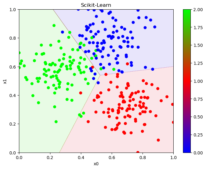
Scikit-Learnの決定境界

model1 = LogisticRegression()
showline_clf(x, y, model1, "Scikit-Learn", x0="x0", x1="x1")

statsmodelsの決定境界

x = sm.add_constant(x)
model2 = sm.MNLogit(y, x).fit_regularized()
showline_clf2(x, y, model2, "statsmodels", x0="x0", x1="x1")

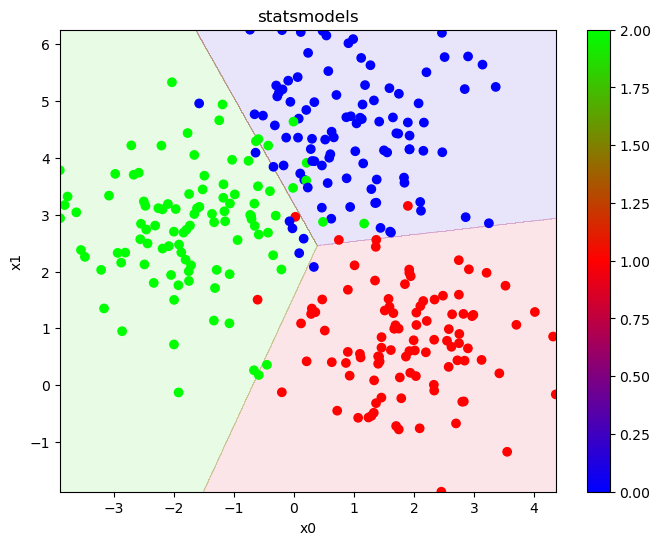
少しだけ決定境界が変わっている事が分かります。
なのでただ予測をする分には切片を追加する事を考慮する事と分類の結果の出力の仕方を追加する以外は特に変わりはありませんが、分析をするとなると少し変わります。

オッズ比の計算

ロジスティック回帰は自然対数に係数乗をするとオッズ比が算出されます。
では実際にオッズ比を見てみましょう。

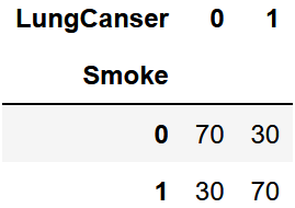
クロス集計表の作成

df = pd.read_csv("LungCanser.csv")
df_cross = pd.crosstab(df["Smoke"], df["LungCanser"])
df_cross

オッズ比の算出

cross = df_cross.values
odds = []
for i in range(len(cross)):
    odds.append(cross[i][1]/cross[i][0])
odds_ratio = ["", odds[1]/odds[0]]
df_odds = pd.DataFrame(odds)
df_odds.columns = ["odds"]
df_odds_ratio = pd.DataFrame(odds_ratio)
df_odds_ratio.columns = ["odds_ratio"]
df_odds = pd.concat([df_odds, df_odds_ratio], axis=1)
df_odds

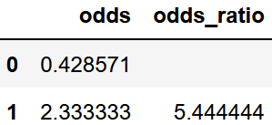
オッズ比は約5.4444となりました。

statsmodelsのロジスティック回帰でオッズ比算出

x = sm.add_constant(df["Smoke"])
y = df["LungCanser"]
model3 = sm.Logit(y, x).fit_regularized()
np.exp(model3.params["Smoke"])

5.444429034587729

一致する値になりました

Scikit-Learnのロジスティック回帰でオッズ比算出

model4 = LogisticRegression()
model4.fit(df["Smoke"].values.reshape(-1, 1), df["LungCanser"])
np.exp(model4.coef_[0][0])

4.707396266875112

先ほどの決定境界の時から分かる通り少し係数が異なるためオッズ比が異なります。

この係数の違いを大きいと見るか小さい誤差と見るかでどちらか楽な方を使えばいいと思いますが、正確な方を使いたいならstatsmodelsになります。

まとめ

統一してよ