タイタニックの質的変数で数量化理論

Kaggleの有名なコンペの一つにタイタニックで生き残る人を見つけるのがあります。
そこには質的変数が非常に多いので質的変数を使って数量化理論をやってみようと思います。

ライブラリのインポート

from sklearn.decomposition import PCA
from sklearn.preprocessing import StandardScaler
import pandas as pd
import statsmodels.api as sm
import numpy as np
import matplotlib.pyplot as plt

データの読み込み

欠損値は下手に代表値で補完すると実データと異なる可能性があるので消します。

df = pd.read_csv("titanic.csv")
df = df.dropna()
df.head()

説明変数選びとダミー変数

質的変数のみ選び必要なものはダミー変数にして量的変数は説明変数から削除します。
また、多重共線性の観点からダミー変数は各一つずつ削除します。

x1 = pd.get_dummies(df.drop(["PassengerId", "Survived","Pclass","Name", "Age", "Fare", "Ticket", "Cabin"], axis=1))
x1 = x1.drop(["Sex_female", "Embarked_C"], axis=1)
x1.head()

数量化理論

数量化理論Ⅰ類

重回帰分析を使います。

年齢を分析

y1 = df["Age"]
model1 = sm.OLS(y1, x1).fit()
model1.summary()

運賃を分析

y2 = df["Fare"]
model2 = sm.OLS(y2, x1).fit()
model2.summary()

数量化理論Ⅱ類

ロジスティック回帰を使います。
生存したかどうかを分析します。

y3 = df["Survived"]
x3 = x1
model3 = sm.Logit(y3, x3).fit_regularized()
model3.summary()

女性が生き残りやすくEmbarkedがSの方が生き残りやすくSibSpが1の人が生き残りやすいそうですね。

数量化理論Ⅲ類

解釈しやすいようにbiplotにします。

x4 = pd.get_dummies(df.drop(["PassengerId", "Survived","Pclass","Name", "Age", "Fare", "Ticket", "Cabin"], axis=1))
col = x4.columns
ss = StandardScaler()
ss.fit(x4)
x4 = ss.transform(x4)
model4 = PCA()
model4.fit(x4)
tx = model4.transform(x4)
exp = model4.explained_variance_ratio_
com = model4.components_
fac = []
for i in range(len(exp)):
    fac.append(np.sqrt(exp[i])*com[i])
fig, ax = plt.subplots()
ax1 = ax.twinx()
ax1.scatter(tx[:, 0], tx[:, 1], c=y3, cmap="brg")
ylim = [abs(max(fac[1])), abs(min(fac[1]))]
xlim = [abs(max(fac[0])), abs(min(fac[0]))]
ax2 = ax.twiny()
for i in range(len(col)):
    ax2.plot([0, fac[0][i]], [0, fac[1][i]], color="#FF0000")
    ax2.text(fac[0][i], fac[1][i], col[i])
ax2.set_xlim(-max(xlim), max(xlim))
ax2.set_ylim(-max(ylim), max(ylim))
plt.show()
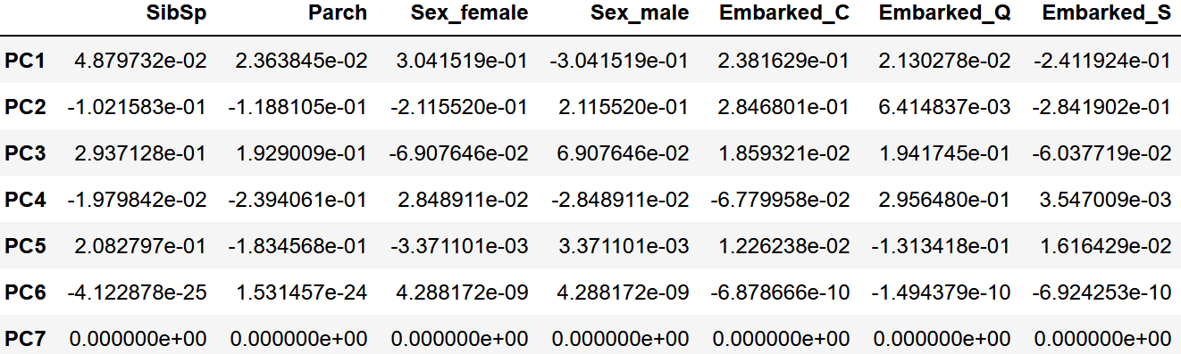
df_fac = pd.DataFrame(fac)
df_fac.columns = col
ind = []
for i in range(len(fac)):
    ind.append("PC%d"%(i+1))
df_fac.index = ind
df_fac

青が生き残れず、緑が生き残れた人です。
Ⅱ類の分析と同様に生き残れた人が女性でEmbarkedがSの方が生き残れやすそうですね。

余談

数量化理論Ⅱ類の精度

from sklearn.metrics import classification_report

pred3 = model3.predict(x3)
y_pred3 = np.where(pred3 >= 0.5, 1, 0)
print(classification_report(y3, y_pred3))

              precision    recall  f1-score   support

           0       0.59      0.70      0.64        60
           1       0.84      0.76      0.80       123

    accuracy                           0.74       183
   macro avg       0.72      0.73      0.72       183
weighted avg       0.76      0.74      0.75       183

意外と74%当たってますね、まあ訓練データとテストデータが同じなので何とも言えませんけど。

LightGBMで予測精度分布

from sklearn.model_selection import train_test_split
from lightgbm import LGBMClassifier

score = []
for i in range(200):
    x_train, x_test, y_train, y_test = train_test_split(x3, y3, random_state=i, test_size=0.3)
    model5 = LGBMClassifier()
    model5.fit(x_train, y_train)
    score.append(model5.score(x_test, y_test))
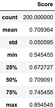
df_scr = pd.DataFrame(score).describe()
df_scr.columns = ["Score"]
df_scr

plt.boxplot(score)
plt.scatter([1],[df_scr.loc["mean", "Score"]])
plt.show()

最大値は外れ値ではないみたいですね。むしろ最小値が外れ値のようです。
いずれにせよ70%の精度が質的変数だけでもあるみたいです。

普通に予測

数量化理論を使わず量的変数も使って予測してみました

score = []
x = pd.get_dummies(df.drop(["PassengerId", "Survived", "Name", "Ticket", "Cabin"], axis=1))
x = x.drop(["Sex_female", "Embarked_C"], axis=1)
y = df["Survived"]
for i in range(200):
    x_train, x_test, y_train, y_test = train_test_split(x, y, random_state=i, test_size=0.3)
    model6 = LGBMClassifier()
    model6.fit(x_train, y_train)
    score.append(model6.score(x_test, y_test))
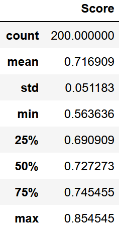
df_scr = pd.DataFrame(score).describe()
df_scr.columns = ["Score"]
df_scr

plt.boxplot(score)
plt.scatter([1],[df_scr.loc["mean", "Score"]], marker="x", color="#000000")
plt.show()

あまり安定していないみたいですが中央値までは精度が向上したみたいです。
なので低い精度は出にくくなったと言えます。ただし精度に限界はあります。

(裏を返せば質的変数が割と目的変数に関連しているのかも)