pytorch3d で python から 3D モデルを表示する

pytorch3d で python から 3D モデルを表示します。

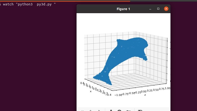
こんな感じで python から 3D モデルの表示を行うことができます（おそらく最適化もできるのかと）

インストール方法

まずは pytorch3d のインストールを行います。環境は Ubuntu になります。

!pip install torch torchvision ;
!pip install 'git+https://github.com/facebookresearch/pytorch3d.git@stable' ;

もし pip のバージョンをアップグレードしてくださいっと言われたら下記コマンドで対応します。

/usr/bin/python3 -m pip install --upgrade pip ;

これで、pytorch3d が使用できる状態になります。

まずは動作確認

メモ帳でも良いですが ubuntu の場合は下記コマンドで新規テキストファイルの作成を行います。

gedit py3d.py ;

コピペするソースコード

py3d.py

mport os
import torch
from pytorch3d.io import load_obj, save_obj
from pytorch3d.structures import Meshes
from pytorch3d.utils import ico_sphere
from pytorch3d.ops import sample_points_from_meshes
from pytorch3d.loss import (
    chamfer_distance,
    mesh_edge_loss,
    mesh_laplacian_smoothing,
    mesh_normal_consistency,
)
import numpy as np
from tqdm.notebook import tqdm
#%matplotlib notebook                                                                                                                                                    
from mpl_toolkits.mplot3d import Axes3D
import matplotlib.pyplot as plt
import matplotlib as mpl
mpl.rcParams['savefig.dpi'] = 80
mpl.rcParams['figure.dpi'] = 80

# Set the device                                                                                                                                                         
if torch.cuda.is_available():
    device = torch.device("cuda:0")
else:
    device = torch.device("cpu")
    print("WARNING: CPU only, this will be slow!")

まずは上記の状態で python を実行します。

python3 py3d.py ;

libcuda が無いよって言われるかと思いますが、これは nvidia のグラフィックボードを搭載していない場合に表示されます。
ライブラリでtensorflowを使う場合は毎回言われるので無視して大丈夫です。 nvidia のグラフィックボードがある場合は計算が早くなります。

次に３Dモデルをダウンロードします。

!wget https://dl.fbaipublicfiles.com/pytorch3d/data/dolphin/dolphin.obj

dolphin、イルカさんですね。

これをソースコードに継ぎ足します。
モデルを読む部分を合算して記載するとこんな感じなります。

py3d.py

import os
import torch
from pytorch3d.io import load_obj, save_obj
from pytorch3d.structures import Meshes
from pytorch3d.utils import ico_sphere
from pytorch3d.ops import sample_points_from_meshes
from pytorch3d.loss import (
    chamfer_distance, 
    mesh_edge_loss, 
    mesh_laplacian_smoothing, 
    mesh_normal_consistency,
)
import numpy as np
from tqdm.notebook import tqdm
#%matplotlib notebook 
from mpl_toolkits.mplot3d import Axes3D
import matplotlib.pyplot as plt
import matplotlib as mpl
mpl.rcParams['savefig.dpi'] = 80
mpl.rcParams['figure.dpi'] = 80

# Set the device
if torch.cuda.is_available():
    device = torch.device("cuda:0")
else:
    device = torch.device("cpu")
    print("WARNING: CPU only, this will be slow!")


# メッシュファイルの読み込み
trg_obj = os.path.join('dolphin.obj')

# 頂点と面とauxの取得
verts, faces, aux = load_obj(trg_obj)
faces_idx = faces.verts_idx.to(device)
verts = verts.to(device)

# (0,0,0)を中心とする半径1の球にフィットするように正規化・中心化
center = verts.mean(0)
verts = verts - center
scale = max(verts.abs().max(0)[0])
verts = verts / scale

# ターゲットメッシュの生成
trg_mesh = Meshes(verts=[verts], faces=[faces_idx])

# ソースメッシュの生成
src_mesh = ico_sphere(4, device)

# メッシュのプロット
def plot_pointcloud(mesh, title=""):
    points = sample_points_from_meshes(mesh, 5000)
    x, y, z = points.clone().detach().cpu().squeeze().unbind(1)
    fig = plt.figure(figsize=(5, 5))
    ax = Axes3D(fig)
    ax.scatter3D(x, z, -y)
    ax.set_xlabel('x')
    ax.set_ylabel('z')
    ax.set_zlabel('y')
    ax.set_title(title)
    ax.view_init(190, 30)
    plt.show()

# ターゲットメッシュとソースメッシュのプロット
plot_pointcloud(trg_mesh, "Target mesh")
plot_pointcloud(src_mesh, "Source mesh")

上記を保存して実行します。

python3 py3d.py ;

毎回このコマンドを打つのが面倒な場合は watch コマンドで定期実行してもよいかと思います。

watch "python3 py3d.py" ;

イルカさんがでるかと思います。

あとは最適化を行います（この辺はよく分かっていません）。
全部のソースコードはこちら。

py3d.py

import os
import torch
from pytorch3d.io import load_obj, save_obj
from pytorch3d.structures import Meshes
from pytorch3d.utils import ico_sphere
from pytorch3d.ops import sample_points_from_meshes
from pytorch3d.loss import (
    chamfer_distance, 
    mesh_edge_loss, 
    mesh_laplacian_smoothing, 
    mesh_normal_consistency,
)
import numpy as np
from tqdm.notebook import tqdm
#%matplotlib notebook 
from mpl_toolkits.mplot3d import Axes3D
import matplotlib.pyplot as plt
import matplotlib as mpl
mpl.rcParams['savefig.dpi'] = 80
mpl.rcParams['figure.dpi'] = 80

# Set the device
if torch.cuda.is_available():
    device = torch.device("cuda:0")
else:
    device = torch.device("cpu")
    print("WARNING: CPU only, this will be slow!")


# メッシュファイルの読み込み
trg_obj = os.path.join('dolphin.obj')

# 頂点と面とauxの取得
verts, faces, aux = load_obj(trg_obj)
faces_idx = faces.verts_idx.to(device)
verts = verts.to(device)

# (0,0,0)を中心とする半径1の球にフィットするように正規化・中心化
center = verts.mean(0)
verts = verts - center
scale = max(verts.abs().max(0)[0])
verts = verts / scale

# ターゲットメッシュの生成
trg_mesh = Meshes(verts=[verts], faces=[faces_idx])

# ソースメッシュの生成
src_mesh = ico_sphere(4, device)

# メッシュのプロット
def plot_pointcloud(mesh, title=""):
    points = sample_points_from_meshes(mesh, 5000)
    x, y, z = points.clone().detach().cpu().squeeze().unbind(1)
    fig = plt.figure(figsize=(5, 5))
    ax = Axes3D(fig)
    ax.scatter3D(x, z, -y)
    ax.set_xlabel('x')
    ax.set_ylabel('z')
    ax.set_zlabel('y')
    ax.set_title(title)
    ax.view_init(190, 30)
    plt.show()

# ターゲットメッシュとソースメッシュのプロット
plot_pointcloud(trg_mesh, "Target mesh")
plot_pointcloud(src_mesh, "Source mesh")

# 変換関数の形状は、src_meshの頂点数と同じ
deform_verts = torch.full(src_mesh.verts_packed().shape, 0.0, device=device, requires_grad=True)

# オプティマイザ
optimizer = torch.optim.SGD([deform_verts], lr=1.0, momentum=0.9)

Niter = 2000 # 最適化ステップの数
w_chamfer = 1.0 # chamfer loss の重み
w_edge = 1.0 # edge lossの重み
w_normal = 0.01 # mesh normal consistencyの重み
w_laplacian = 0.1 # mesh laplacian smoothingの重み
plot_period = 250 # プロット頻度
loop = tqdm_notebook(range(Niter))

chamfer_losses = []
laplacian_losses = []
edge_losses = []
normal_losses = []

#%matplotlib inline

for i in loop:
    # オプティマイザの初期化
    optimizer.zero_grad()

    # メッシュの変形
    new_src_mesh = src_mesh.offset_verts(deform_verts)

    # 各メッシュの表面から5000個の点をサンプリング
    sample_trg = sample_points_from_meshes(trg_mesh, 5000)
    sample_src = sample_points_from_meshes(new_src_mesh, 5000)

    # chamfer loss
    loss_chamfer, _ = chamfer_distance(sample_trg, sample_src)

    # edge loss
    loss_edge = mesh_edge_loss(new_src_mesh)

    # normal loss
    loss_normal = mesh_normal_consistency(new_src_mesh)

    # laplacian loss
    loss_laplacian = mesh_laplacian_smoothing(new_src_mesh, method="uniform")

    # 損失の加重合計
    loss = loss_chamfer * w_chamfer + loss_edge * w_edge + loss_normal * w_normal + loss_laplacian * w_laplacian

    # 損失の出力
    loop.set_description('total_loss = %.6f' % loss)

    # プロットのための損失の保存
    chamfer_losses.append(loss_chamfer)
    edge_losses.append(loss_edge)
    normal_losses.append(loss_normal)
    laplacian_losses.append(loss_laplacian)

    # メッシュのプロット
    if i % plot_period == 0:
        plot_pointcloud(new_src_mesh, title="iter: %d" % i)

    # 最適化ステップ
    loss.backward()
    optimizer.step()

公式サイト にはテクスチャを貼ったものや反射しているものもあるので、レンダリングソフトとしても面白いかもしれません。

参考リンク

• facebookresearch/pytorch3d: PyTorch3D is FAIR's library of reusable components for deep learning with 3D data
• PyTorch3D 入門｜npaka｜note
• pytorch3d/deform_source_mesh_to_target_mesh.ipynb at master · facebookresearch/pytorch3d