はじめに
やりたいことは python3 で時系列分析を行い、予測までしてみること。
特に季節変動を加味したSARIMAモデルを扱ってみたい。
利用するデータとしては、以下の参考資料で、TV朝日の視聴率の時系列分析をしてみる。
きっかけは2016年度4Qで大きく利益率を落としているが、視聴率変動がどう影響しているのか、今後の変動はどう予測できるのかを試行した。
参考資料
http://www.tv-asahihd.co.jp/contents/ir_setex/
未来を予測するビッグデータの解析手法と「SARIMAモデル」 - DeepAge
https://deepage.net/bigdata/2016/10/22/bigdata-analytics.html
SARIMA モデルの概要
SARIMAモデルは複数の時系列モデルを複合した手法。
以下の図のような関係があります。
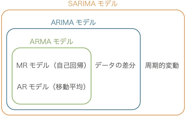
(出典: 未来を予測するビッグデータの解析手法と「SARIMAモデル」 - DeepAge)
ARモデル(自己回帰モデル, autoregressive model)
ARモデルは図のように時間の変化に対し規則的に値が変化する、最も単純な時系列モデル。
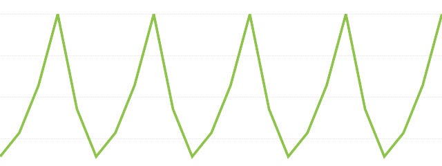
直前のp個の値と相関のあるモデルをAR(p)と表現します。
ARモデルはある時点のデータがそれ以前のデータで回帰的に推定できるモデルです。
MAモデル(移動平均モデル、Moving Average model)
MAモデルは図のように時間の変化に対し不規則に値が変化するけど、
ある区間での変動が一定であるようにモデルを考えます。
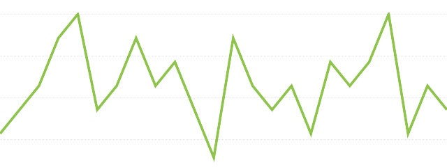
直前のq個の値の誤差の影響を受けるモデルをMA(q)と表現します。
MAモデルは過去の誤差に影響されるモデルです。
ARMAモデル(自己回帰移動平均モデル)
ARモデルとMAモデルの2つ組み合わせて定式化したモデル。
ARモデルに関連する次数をpとMAモデルに関連する次数をqとすると、ARMA(p,q)と表すことができます。
定常性
ARモデル、MAモデル、ARMAモデルはいずれも定常過程を対象とした時系列モデル。
定常過程は、以下の二つを満たすものを言います。
・平均が時間に依存せずに一定である
・異時点間の共分散が時間差のみに依存する
つまり、定常性のある時系列データは「一定の周期で同程度の変動をしている」といえます。
時系列において、平均値が時間的に常に一定であることが保証されているのは稀。
つまり現実に扱う時系列データは非定常過程であることが多い。
実用に際しては、非定常過程の時系列データを対象とした手法を用いる必要があります。
そこで、SARIMAの出番です。
SARIMAモデル(季節自己回帰和分移動平均モデル)
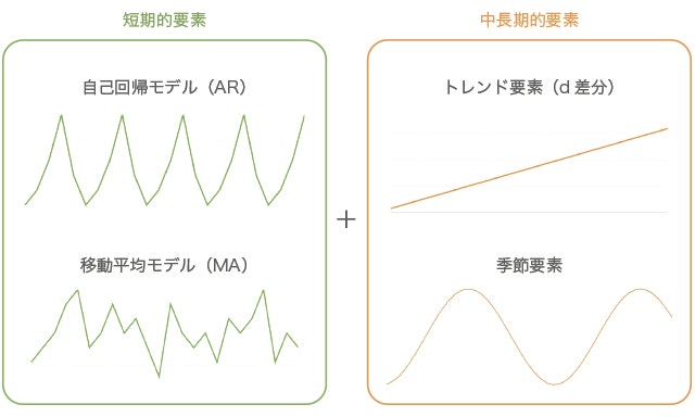
(出典: 未来を予測するビッグデータの解析手法と「SARIMAモデル」 - DeepAge)
最後は少しはしょりましたが、本題にGo.
データを準備する
# 基本のライブラリを読み込む
import numpy as np
import pandas as pd
from scipy import stats

# グラフ描画
from matplotlib import pylab as plt
import seaborn as sns
%matplotlib inline


# グラフを横長にする
from matplotlib.pylab import rcParams
rcParams['figure.figsize'] = 15, 6

import matplotlib as mpl
mpl.rcParams['font.family'] = ['serif']

url = "/work/02_timeseries/tvasahi201701.txt"
file2 = "/work/02_timeseries/tvasahi201701_2.txt"
dataNormal = pd.read_csv(url)
dataNormal.head()

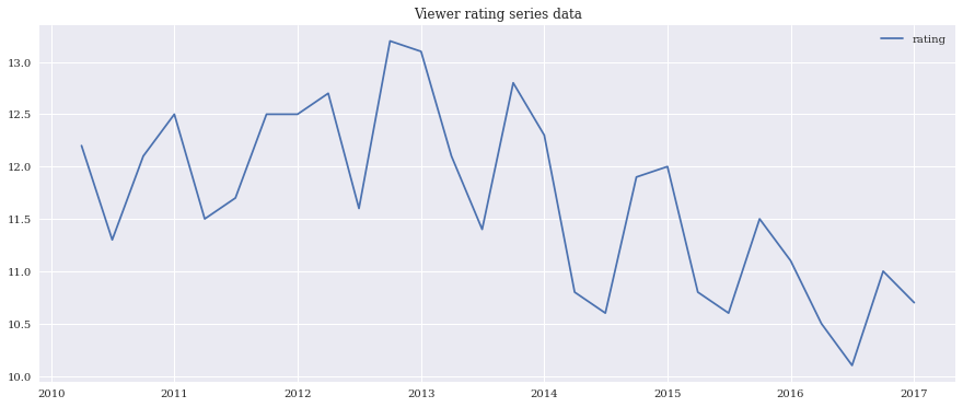
全日、ゴールデン、プライム、プライム2の時間帯で視聴率データが揃えられる。
今回はプライムタイムのみのデータを利用して分析してみる。なぜこのデータをチョイスしたかというとトレンドがはっきり現れていて、データ分析、予測の学習にはもってこいだから。
まず、このデータをプロットしてみる。
ts = ((dataNormal.T)[2])

dateparse = lambda dates: pd.datetime.strptime(dates, '%Y-%m-01')
ts = pd.read_csv(file2, index_col="time", date_parser=dateparse, dtype='float')
plt.plot(ts, label='rating')
plt.title('Viewer rating series data')
plt.legend(loc='best')
Dickey-Fuller test
定常性をチェックするための統計的テストの1つです。
ここで、帰無仮説は、ts が非定常であるということ。
テスト結果は、「検定統計量(Test Statistic)」と1,5,10%の信頼水準の「臨界値(Critical Value)」から構成されます。
「検定統計量」が「臨界値」よりも小さい場合は、帰無仮説を棄却して系列が定常状態と判定できます。
from statsmodels.tsa.stattools import adfuller
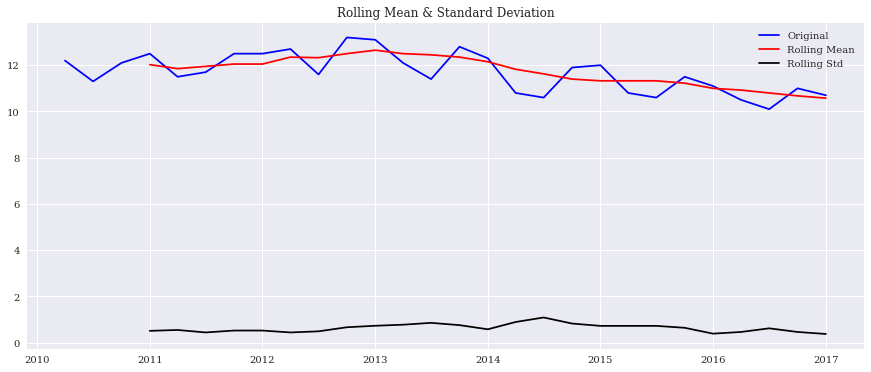
# Dickey-Fuller test 結果と標準偏差、平均のプロット
def test_stationarity(timeseries, window_size=12):
# Determing rolling statistics
rolmean = timeseries.rolling(window=window_size,center=False).mean()
rolstd = timeseries.rolling(window=window_size,center=False).std()
# Plot rolling statistics:
orig = plt.plot(timeseries, color='blue',label='Original')
mean = plt.plot(rolmean, color='red', label='Rolling Mean')
std = plt.plot(rolstd, color='black', label = 'Rolling Std')
plt.legend(loc='best')
plt.title('Rolling Mean & Standard Deviation')
plt.show(block=False)
# Perform Dickey-Fuller test:
print('Results of Dickey-Fuller Test:')
dftest = adfuller(timeseries, autolag='AIC')
dfoutput = pd.Series(dftest[0:4], index=['Test Statistic','p-value',
'#Lags Used','Number of Observations Used'])
for key,value in dftest[4].items():
dfoutput['Critical Value (%s)'%key] = value
print(dfoutput)
まずは上記関数を呼び出してみる。
test_stationarity(ts, window_size=4)
Results of Dickey-Fuller Test:
---------------------------------------------------------------------------
ValueError                                Traceback (most recent call last)
<ipython-input-8-552a0eb0606f> in <module>()
----> 1 test_stationarity(ts, window_size=4)

<ipython-input-7-e5ce27c1c7e1> in test_stationarity(timeseries, window_size)
     17     # Perform Dickey-Fuller test:
     18     print('Results of Dickey-Fuller Test:')
---> 19     dftest = adfuller(timeseries, autolag='AIC')
     20     dfoutput = pd.Series(dftest[0:4], index=['Test Statistic','p-value',
     21                                              '#Lags Used','Number of Observations Used'])

/root/anaconda3/lib/python3.6/site-packages/statsmodels/tsa/stattools.py in adfuller(x, maxlag, regression, autolag, store, regresults)
    218
    219     xdiff = np.diff(x)
--> 220     xdall = lagmat(xdiff[:, None], maxlag, trim='both', original='in')
    221     nobs = xdall.shape[0]  # pylint: disable=E1103
    222

/root/anaconda3/lib/python3.6/site-packages/statsmodels/tsa/tsatools.py in lagmat(x, maxlag, trim, original, use_pandas)
    373     if xa.ndim == 1:
    374         xa = xa[:, None]
--> 375     nobs, nvar = xa.shape
    376     if original in ['ex', 'sep']:
    377         dropidx = nvar

ValueError: too many values to unpack (expected 2)
エラーが出てしまいました。
標準偏差は大きく変動していないけど、移動平均は緩やかに下落している模様。
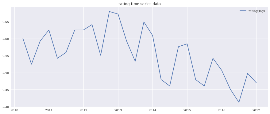
対数をとって傾向を確認
次に対数をとって傾向を確認して見ましょう。
ts_log = np.log(ts)
plt.plot(ts_log, label='rating(log)')
plt.title('rating time series data')
plt.legend(loc='best')
次に対数データについて、傾向、季節性、残差を眺めてみる。
# 傾向(trend)、季節性(seasonal)、残差(residual)に分解してモデル化する。
from statsmodels.tsa.seasonal import seasonal_decompose
decomposition = seasonal_decompose(ts_log)

trend = decomposition.trend
seasonal = decomposition.seasonal
residual = decomposition.resid


# オリジナルの時系列データプロット
plt.subplot(411)
plt.plot(ts_log, label='Original')
plt.legend(loc='best')

# trend のプロット
plt.subplot(412)
plt.plot(trend, label='Trend')
plt.legend(loc='best')

# seasonal のプロット
plt.subplot(413)
plt.plot(seasonal,label='Seasonality')
plt.legend(loc='best')

# residual のプロット
plt.subplot(414)
plt.plot(residual, label='Residuals')
plt.legend(loc='best')
plt.tight_layout()
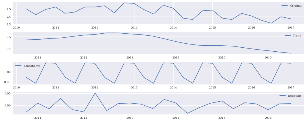
秋にかけて視聴率が下がり、冬に視聴率が上がるというのが毎年の季節性のある傾向。
トレンドとしては緩やかに下がってきているのが見て取れます。
SARIMAモデルの最適なパラメータを探す
SARIMA モデルを以下のライブラリでオブジェクト化してみるが、
http://www.statsmodels.org/dev/generated/statsmodels.tsa.statespace.sarimax.SARIMAX.html
sarima = sm.tsa.SARIMAX(
    ts, order=(p,d,q),
    seasonal_order=(sp,sd,sq,4),
    enforce_stationarity = False,
    enforce_invertibility = False)
p,d,q,sp,sd,sq の組み合わせを探してみる。
(sp,sd,sq,4)の最後の4は年間を四半期に分けているので分割数4と指定しています。
import statsmodels.api as sm

# 自動SARIMA選択
num = 0

for p in range(1, max_p + 1):
    for d in range(0, max_d + 1):
        for q in range(0, max_q + 1):
            for sp in range(0, max_sp + 1):
                for sd in range(0, max_sd + 1):
                    for sq in range(0, max_sq + 1):
                        sarima = sm.tsa.SARIMAX(
                            ts, order=(p,d,q),
                            seasonal_order=(sp,sd,sq,4),
                            enforce_stationarity = False,
                            enforce_invertibility = False
                        ).fit()
                        modelSelection.iloc[num]["model"] = "order=(" + str(p) + ","+ str(d) + ","+ str(q) + "), season=("+ str(sp) + ","+ str(sd) + "," + str(sq) + ")"
                        modelSelection.iloc[num]["aic"] = sarima.aic
                        num = num + 1

# モデルごとの結果確認
print(modelSelection)

# AIC最小モデル
print(modelSelection[modelSelection.aic == min(modelSelection.aic)])
以下が実行結果。
                           model      aic
0    order=(1,0,0), season=(0,0,0)  70.3877
1    order=(1,0,0), season=(0,0,1)  48.7876
2    order=(1,0,0), season=(0,1,0)  40.1175
3    order=(1,0,0), season=(0,1,1)  27.9964
4    order=(1,0,0), season=(1,0,0)   40.728
5    order=(1,0,0), season=(1,0,1)  37.2894
6    order=(1,0,0), season=(1,1,0)  30.3103
7    order=(1,0,0), season=(1,1,1)   29.522
8    order=(1,0,1), season=(0,0,0)  62.5256
9    order=(1,0,1), season=(0,0,1)  43.3847
10   order=(1,0,1), season=(0,1,0)  37.7301
11   order=(1,0,1), season=(0,1,1)  26.0388
12   order=(1,0,1), season=(1,0,0)  41.8186
13   order=(1,0,1), season=(1,0,1)  32.2768
14   order=(1,0,1), season=(1,1,0)  31.8695
15   order=(1,0,1), season=(1,1,1)  28.0252
16   order=(1,0,2), season=(0,0,0)  57.7646
17   order=(1,0,2), season=(0,0,1)  40.7138
18   order=(1,0,2), season=(0,1,0)  36.0716
19   order=(1,0,2), season=(0,1,1)  25.3384
20   order=(1,0,2), season=(1,0,0)  42.2375
21   order=(1,0,2), season=(1,0,1)  28.2212
22   order=(1,0,2), season=(1,1,0)  33.8669
23   order=(1,0,2), season=(1,1,1)  27.4596
24   order=(1,0,3), season=(0,0,0)    57.36
25   order=(1,0,3), season=(0,0,1)  39.7003
26   order=(1,0,3), season=(0,1,0)  37.0603
27   order=(1,0,3), season=(0,1,1)    24.85
28   order=(1,0,3), season=(1,0,0)  45.7587
29   order=(1,0,3), season=(1,0,1)  30.5274
..                             ...      ...
162  order=(3,1,0), season=(0,1,0)  35.6774
163  order=(3,1,0), season=(0,1,1)  26.6998
164  order=(3,1,0), season=(1,0,0)  36.7483
165  order=(3,1,0), season=(1,0,1)  37.3619
166  order=(3,1,0), season=(1,1,0)  27.1641
167  order=(3,1,0), season=(1,1,1)  23.5206
168  order=(3,1,1), season=(0,0,0)  46.0088
169  order=(3,1,1), season=(0,0,1)  42.0283
170  order=(3,1,1), season=(0,1,0)  33.2783
171  order=(3,1,1), season=(0,1,1)  23.3888
172  order=(3,1,1), season=(1,0,0)  33.2987
173  order=(3,1,1), season=(1,0,1)  34.8924
174  order=(3,1,1), season=(1,1,0)  24.7505
175  order=(3,1,1), season=(1,1,1)  25.6202
176  order=(3,1,2), season=(0,0,0)  40.3796
177  order=(3,1,2), season=(0,0,1)  37.4187
178  order=(3,1,2), season=(0,1,0)  35.7897
179  order=(3,1,2), season=(0,1,1)  23.3374
180  order=(3,1,2), season=(1,0,0)  38.7358
181  order=(3,1,2), season=(1,0,1)  37.6919
182  order=(3,1,2), season=(1,1,0)  29.2141
183  order=(3,1,2), season=(1,1,1)  27.3448
184  order=(3,1,3), season=(0,0,0)  41.1869
185  order=(3,1,3), season=(0,0,1)  34.1721
186  order=(3,1,3), season=(0,1,0)  34.8843
187  order=(3,1,3), season=(0,1,1)  23.1797
188  order=(3,1,3), season=(1,0,0)  40.3741
189  order=(3,1,3), season=(1,0,1)  35.8745
190  order=(3,1,3), season=(1,1,0)  23.1581
191  order=(3,1,3), season=(1,1,1)  29.1668

[192 rows x 2 columns]
                            model      aic
59  order=(1,1,3), season=(0,1,1)  20.1616
「order=(1,1,3), season=(0,1,1)」が最適なパラメータらしいので、
このパラメータでSARIMAモデルを作成する。
p=1
d=1
q=3
sp=0
sd=1
sq=1

sarima = sm.tsa.SARIMAX(
    ts, order=(p,d,q),
    seasonal_order=(sp,sd,sq,4),
    enforce_stationarity = False,
    enforce_invertibility = False
).fit()
# 結果確認
print(sarima.summary())
 Statespace Model Results
=========================================================================================
Dep. Variable:                              プライム   No. Observations:                   28
Model:             SARIMAX(1, 1, 3)x(0, 1, 1, 4)   Log Likelihood                  -4.081
Date:                           Sat, 26 Aug 2017   AIC                             20.162
Time:                                   10:16:53   BIC                             28.155
Sample:                               04-01-2010   HQIC                            22.605
                                    - 01-01-2017
Covariance Type:                             opg
==============================================================================
                 coef    std err          z      P>|z|      [0.025      0.975]
------------------------------------------------------------------------------
ar.L1          0.7597   2.03e+06   3.74e-07      1.000   -3.99e+06    3.99e+06
ma.L1         -1.2405      0.000  -5216.846      0.000      -1.241      -1.240
ma.L2         -0.0121      0.003     -4.468      0.000      -0.017      -0.007
ma.L3          0.2525      0.011     22.090      0.000       0.230       0.275
ma.S.L4       -1.0001      0.013    -77.808      0.000      -1.025      -0.975
sigma2         0.0624      0.015      4.218      0.000       0.033       0.091
===================================================================================
Ljung-Box (Q):                        5.47   Jarque-Bera (JB):                 0.47
Prob(Q):                              0.98   Prob(JB):                         0.79
Heteroskedasticity (H):               0.21   Skew:                            -0.43
Prob(H) (two-sided):                  0.11   Kurtosis:                         3.02
===================================================================================

Warnings:
[1] Covariance matrix calculated using the outer product of gradients (complex-step).
[2] Covariance matrix is singular or near-singular, with condition number 2.18e+36. Standard errors may be unstable.
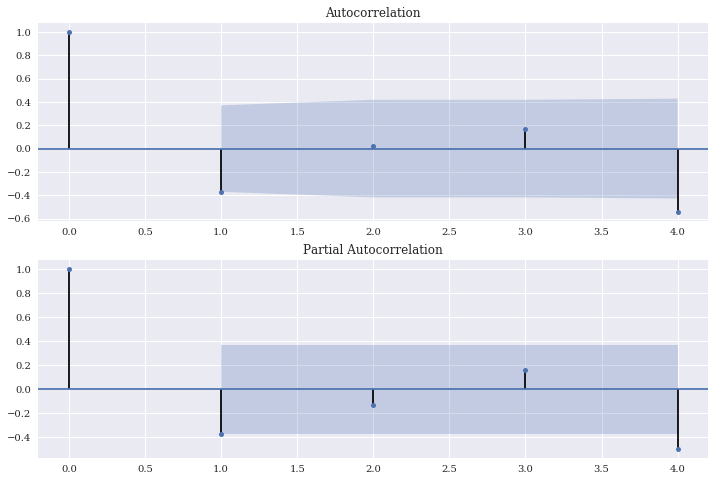
# 残差のチェック
residSARIMA = sarima.resid
fig = plt.figure(figsize=(12,8))

# 自己相関
ax1 = fig.add_subplot(211)
fig = sm.graphics.tsa.plot_acf(residSARIMA, lags=4, ax=ax1)

# 偏自己相関
ax2 = fig.add_subplot(212)
fig = sm.graphics.tsa.plot_pacf(residSARIMA, lags=4, ax=ax2)
残差の自己相関については、ほぼ問題なくなったことを確認。
最後に予測
長々と色々見てきましたが、SARIMA モデルでどれだけ予測できるのかを見てみます。
元データは2010年1Qから2016年4Qですが、この元データと予測データ(2015年1Q-2017年4Q)までを同時プロットしてみます。
# 予測
ts_pred = sarima.predict('2015-01-01', '2017-12-01')

# 実データと予測結果の図示
plt.plot(ts, label='original')
plt.plot(ts_pred, label='predicted', color='red')
plt.legend(loc='best')

print(ts_pred)
2015-01-01    11.601939
2015-04-01    10.927707
2015-07-01    10.164144
2015-10-01    11.711078
2016-01-01    11.266165
2016-04-01    10.183324
2016-07-01     9.949642
2016-10-01    11.106567
2017-01-01    10.775023
2017-04-01     9.803198
2017-07-01     9.344881
2017-10-01    10.452862
Freq: QS-OCT, dtype: float64
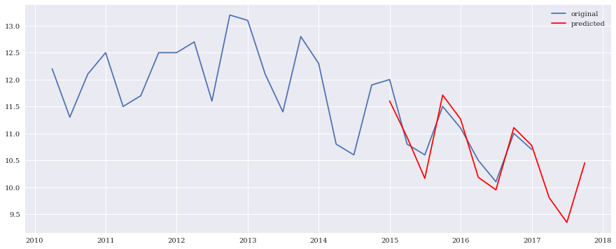
2015-2016年度のデータはまずまずの精度で予測できていることが分かります。
2017年度は秋口にかけて大きく下落し、冬に大きく上昇することが予測できそう。
トレンドを加味して予測するのはさほど難しくないですね。
今回はcost function による厳密なcost分析を行っていませんが、
今後のアンサンブル解析時の課題としたいと思います。
今回の解析notebook
今回の詳細データ解析過程については notebook を参照してください。
https://github.com/mshinoda88/python/blob/master/20170822-01_tvasahi.ipynb