(途中)外サイクロイド<1/2>「2022 産業医科大学 医学部【3】」をWolframAlphaとsympyでやってみたい。

(2023-10-23タイトル変更済み)

パイソニスタの方へ アドバイスをいただけると助かります。
①(コードあり)sympyのplot関数のextendのループの仕方を教えて下さい。
　複数個、配列です。
②plot関数をdashにするには、バックグラウンド?を使うしか方法がありませんか？
③plot関数のx軸メモリの位置を、一番下へ移動したい。現在中央です。
よろしくお願いします。

オリジナル

大学入試数学問題集成 様＞テキスト【3】

WolframAlphaで

・sympyの計算式で、作図しました。

sympyで(抜粋)"セ"から"ツ"までです。

　
・ソースコードは,図2',図1'の順番です。申し訳ありません(ver0.1)
・ｎ本の折れ線を関数にしたいです。

・sympy.plotting.plot.plot_parametric(*args, show=True, **kwargs)
https://docs.sympy.org/latest/modules/plotting.html#sympy.plotting.plot.plot_parametric

# ver0.1
from sympy import *
var('f,a,b',real=True,nonnegative=True)
var('θ1,θ2',real=True,nonnegative=True)
var('ω1,ω2',real=True,nonnegative=True)
var('t,Φ'  ,real=True,nonnegative=True)
(Tp,a,b,f)=(1,2,1,5)
O=Point(0,0)
# ------------------------------------------------------------------
P=(Point(f,0)+Point(a*cos(θ1),a*sin(θ1)))
S=(P         +Point(b*cos(θ2),b*sin(θ2)))
print("#セ",P)
print("#ソ",S)
# ------------------------------------------------------------------
rep_θt={θ1:ω1*t,θ2:ω2*t+Φ}
print("#タ",solve(Eq(2*pi,ω1*Tp),Tp)[0])
# ------------------------------------------------------------------
(P,S)=(P.subs(rep_θt),S.subs(rep_θt))
PS   =O.distance(P)-O.distance(S)
Φ_sol=solveset( Eq(PS.subs({t:0}),1),Φ,Interval(0,2*pi)).args[0]
ω1_sol=(            2 *pi)/Tp
ω2_sol=(Rational(10,2)*pi)/Tp   #回転2.5倍(=5÷2)
print("#チ",ω1_sol)
print("#チ",ω2_sol)
print("#ツ", Φ_sol)
#########################################################################
# 図2'------------------------------------------------------------------
Pt=(O.distance(P)).subs({ω1:ω1_sol})
St=(O.distance(S)).subs({ω1:ω1_sol,ω2:ω2_sol,Φ:Φ_sol})
tHani=(t,0,1.5)
pl_Pt=plot(Pt,tHani,show=False,aspect_ratio=(5.0,1.0),ylim=(2,9))
pl_St=plot(St,tHani,show=False)
pl_Pt.extend(pl_St)
pl_Pt.show()
# 図1'------------------------------------------------------------------
P=(Point(f,0)+Point(a*cos(θ1),a*sin(θ1))).subs(rep_θt).subs({ω1:ω1_sol,ω2:ω2_sol,Φ:Φ_sol})
S=(P         +Point(b*cos(θ2),b*sin(θ2))).subs(rep_θt).subs({ω1:ω1_sol,ω2:ω2_sol,Φ:Φ_sol})
(st,en)=(0,1.0)
ax1=plot_parametric(P.x,P.y,(t,st,en),aspect_ratio=(1.0,1.0),
                    # line_color="blue",
                    show=False
                  )
ax2=plot_parametric(S.x,S.y,(t,st,en),
                    # line_color="blue",
                    show=False
                  )
# ------------------------------------------------------------------
def myPlotLineOPS1(tOP,O,P,S):
    var('u'  ,real=True)
    OPu=O+u*Point(P.x,P.y).subs({t:tOP})
    PSu=  1*Point(P.x,P.y).subs({t:tOP})+u*Point(S.x-P.x,S.y-P.y).subs({t:tOP})
    ay1=plot_parametric(PSu.x,PSu.y,(u,0,1),line_color="black",
                        show=False
                       )
    return ay1
def myPlotLineOPS2(tOP,O,P,S):
    var('u'  ,real=True)
    OPu=O+u*Point(P.x,P.y).subs({t:tOP})
    PSu=  1*Point(P.x,P.y).subs({t:tOP})+u*Point(S.x-P.x,S.y-P.y).subs({t:tOP})
    ay2=plot_parametric(PSu.x,PSu.y,(u,0,1),line_color="black",
                        show=False
                       )
    return ay2
def myPlotLineOPS4(tOP,O,P,S):
    var('u'  ,real=True)
    OPu=O+u*Point(P.x,P.y).subs({t:tOP})
    PSu=  1*Point(P.x,P.y).subs({t:tOP})+u*Point(S.x-P.x,S.y-P.y).subs({t:tOP})
    ay4=plot_parametric(PSu.x,PSu.y,(u,0,1),line_color="black",
                        show=False
                       )
    return ay4
def myPlotLineOPS6(tOP,O,P,S):
    var('u'  ,real=True)
    OPu=O+u*Point(P.x,P.y).subs({t:tOP})
    PSu=  1*Point(P.x,P.y).subs({t:tOP})+u*Point(S.x-P.x,S.y-P.y).subs({t:tOP})
    ay6=plot_parametric(PSu.x,PSu.y,(u,0,1),line_color="black",
                        show=False
                       )
    return ay6
ax1.extend(ax2)
ax1.extend(myPlotLineOPS1(0.1,O,P,S))
ax1.extend(myPlotLineOPS2(0.2,O,P,S))
ax1.extend(myPlotLineOPS4(0.4,O,P,S))
ax1.extend(myPlotLineOPS6(0.6,O,P,S))
ax1.show()
#セ Point2D(2*cos(θ1) + 5, 2*sin(θ1))
#ソ Point2D(2*cos(θ1) + cos(θ2) + 5, 2*sin(θ1) + sin(θ2))
#タ 2*pi/ω1
#チ 2*pi
#チ 5*pi
#ツ pi

図1'

軌跡平面図抜粋 2.5倍でいいですか?

・黒360°回転するところで、青が144°回転する。 2.5倍に見えますか？
　ω1,ω2定数。角速度? 　(0≦t≦1.0)
・黒色は、線分PSの抜粋です。線分A、線分B省略。(線の色,細さ勉強中。)

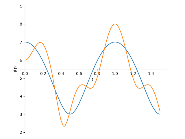
図2'

・以下のグラフから、2.5倍と読み取る方法を教えて下さい。
　赤本が楽しみです。
・横軸が時間tで、縦軸が原点から,点P,Qへの距離です。

いつもの? sympyの実行環境と 参考のおすすめです。

(テンプレート)

(以下テストです)作業用

＜ 大学入試数学問題集成掲示板　2023/10/18 (Wed) 22:26:27
https://mathexamtest.bbs.fc2.com/

参考式から

B=root((2cos2pix +5+cos(pix-pi)^2+(2sin2pix　+cos(pix-pi)^2)
√ ((2cos2πx +5+cos(πx-π) ^2+(2sin2πx 　+cos(πx-π) ^2)
√ ((2cos(2πx)+5+cos(πx-π)) ^2+(2sin(2πx)+cos(πx-π)) ^2)
√ ((2cos(2πx)+5+cos(πx-π)) ^2+(2sin(2πx)+cos(πx-π)) ^2),0≦x≦1.5,グラフ

私の式

wollframを見て下さい。

黄色が参考式

??? わかりませんでした。???

(抜粋)以下は単独で、動作しません
pMeta=plot(sqrt((2*cos(2*pi*t)+5+cos(pi*t-pi)) **2+(2*sin(2*pi*t)+cos(pi*t-pi))**2),
             tHani,show=False,line_color="yellow",) 
pl_Pt.extend(pl_St)

次頁<２/2>点Pが2周します。へ続く