はじめに

前回に引き続き、Rのデータ解析の勉強会に出席しました
今回は時系列データです、Pythonだとどうするの？を復習を兼ねて記録に残したいと思います
かなり不満足な結果となりましたが、統計の専門ではない人間がサクッと調べた結果ということで
RとPython（の統計関係のライブラリー充実度かな？）の違いを実感しました
Rは統計関係充実していますね~

環境

windows10 Pro 64bit
R :3.6.1
RStudio :1.2.1335

Google Colaboratoryを使用
Python :3.6.8

何するの？

Rに実装されている？データセットUKgasを用いて時系列データ解析を行う

①差分データをプロットしてみる
②対数にしてみる
③自己相関関数（acf:autocorrelation function)で周期性を見てみる
④スペクトル分析をしてみる
⑤単位根検定をしてみる
⑥ARモデル（自己回帰モデル）を見てみる
　　独立性検定　Box-Pierce検定をしてみる
　　正規性検定　Ljung-Box検定をしてみる
　　予測をしてみる
⑦差分を対数にしてARモデルを試す
⑧ARMAモデル（自己回帰移動平均モデル）を試してみる

Rのコード

データセットの読み込みと確認


#データの読み込み
data(UKgas)

class(UKgas)#データ形式の確認　ts 時系列 (time series) 
[1] "ts"

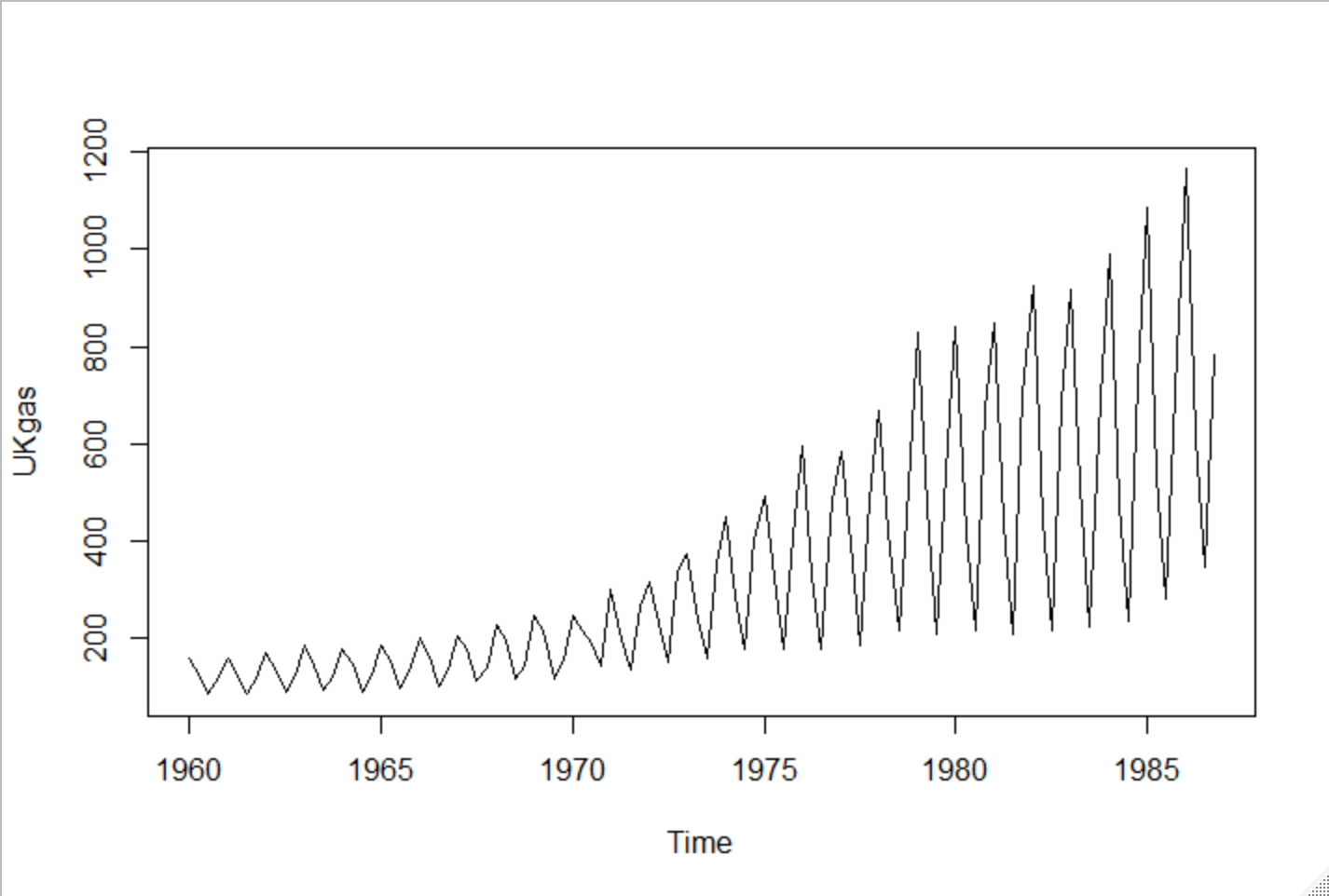
UKgas#1960年から1986年までの四半期ごとのガスの使用量？

      Qtr1   Qtr2   Qtr3   Qtr4
1960  160.1  129.7   84.8  120.1
1961  160.1  124.9   84.8  116.9
...
1985 1087.0  534.7  281.8  787.6
1986 1163.9  613.1  347.4  782.8

生データプロット

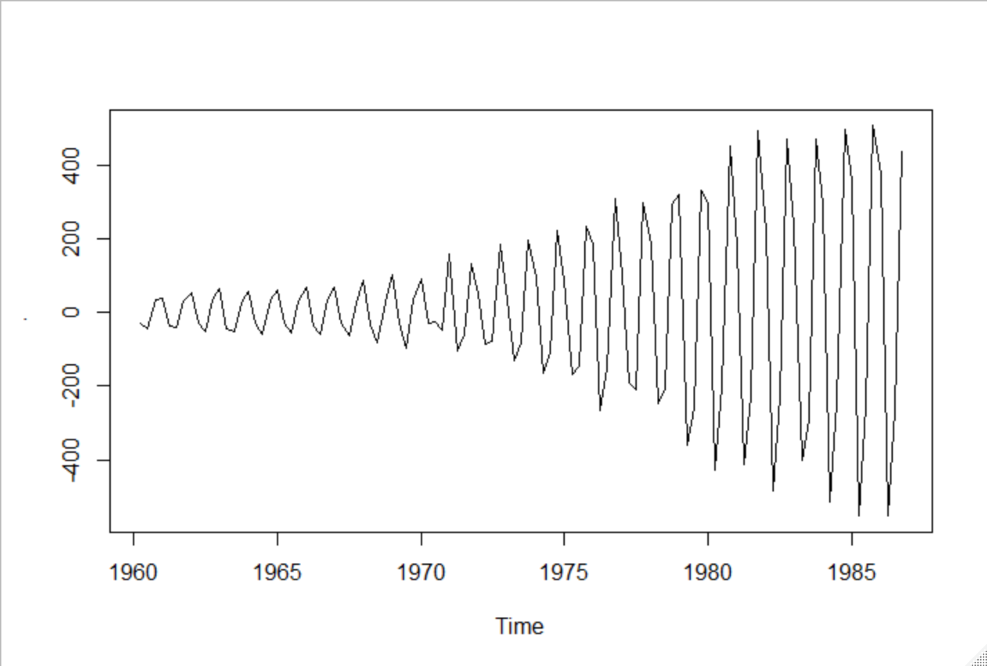
①差分データをプロット

UKgas %>% diff() %>% plot()

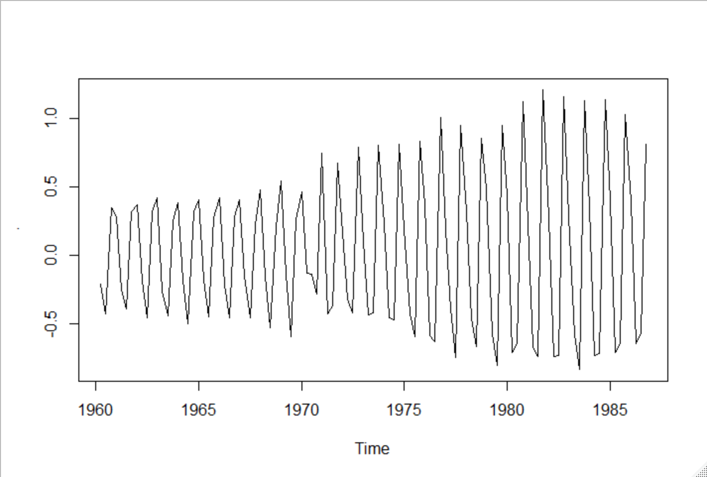
②対数でプロット

UKgas %>% log() %>% diff() %>% plot()

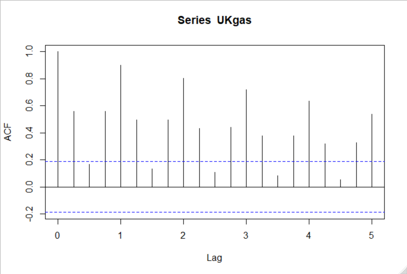
③自己相関関数で周期性を見てみる

acf(UKgas)
1年単位で自己相関が高く、周期性がみられる
Lag0は自分自身との相関なので相関係数1

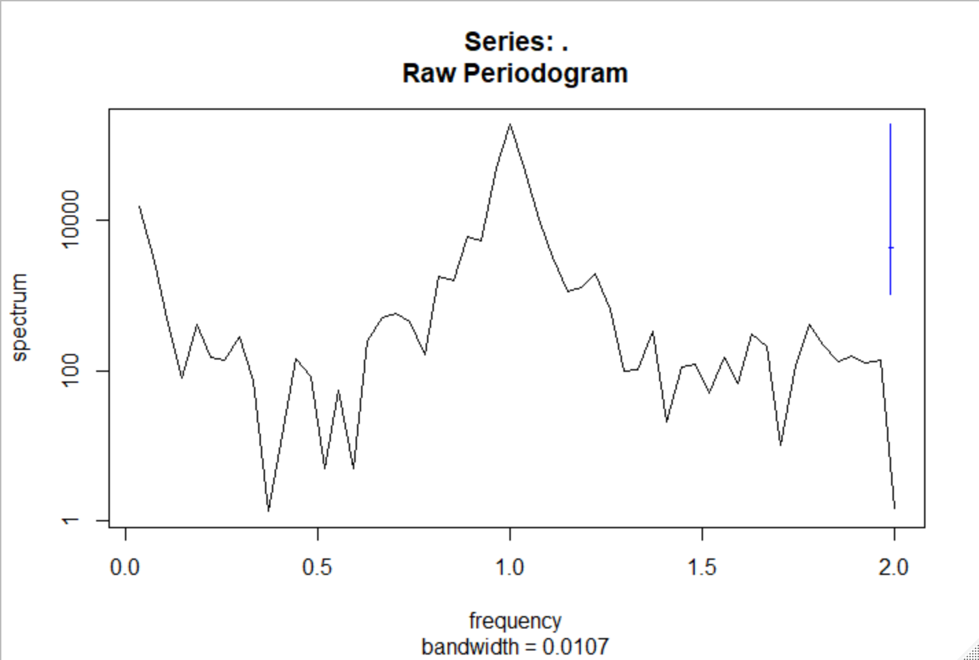
④スペクトル分析をしてみる

1.0に周期がありますね
UKgas %>% spec.pgram()

⑤単位根検定をしてみる

時系列が単位根を持つかどうか（ランダムウォークであるか）を調べること
単位根検定とは、「|a| = 1」であるという帰無仮説検定である。

Phillips-Perron 検定
p値が0.01なので、単位根があるという帰無仮説が棄却される


PP.test(UKgas)

    Phillips-Perron Unit Root Test

data:  UKgas
Dickey-Fuller = -10.126, Truncation lag parameter = 4, p-value = 0.01

Augmented Dickey-Fuller 検定
（対立仮説は「|a| < 1 (stationary)」か「|a| > 1 (explosive)」を選択できる）

stationary：p値が0.73なので棄却できない
explosive：p値が0.26なので棄却できない
あれ？困ったぞ


adf.test(UKgas)

Augmented Dickey-Fuller Test

data:  UKgas
Dickey-Fuller = -1.6079, Lag order = 4, p-value = 0.7393
alternative hypothesis: stationary


adf.test(UKgas,alternative = "explosive")

Augmented Dickey-Fuller Test

data:  UKgas
Dickey-Fuller = -1.6079, Lag order = 4, p-value = 0.2607
alternative hypothesis: explosive

差分データで検定してみると棄却できた！


adf.test(diff(UKgas))

data:  diff(UKgas)
Dickey-Fuller = -7.1679, Lag order = 4, p-value = 0.01
alternative hypothesis: stationary

Warning message:
In adf.test(diff(UKgas)) : p-value smaller than printed p-value

⑥ARモデル（自己回帰モデル）を見てみる

ARモデルの係数を算出
独立性検定　Box-Pierce検定、Ljung-Box検定をしてみる
　　p値が0.1378なので独立性があるとは言い切れない、相関関係がありそう
正規性検定　ジャック・ベラ検定検定をしてみる
　　P値が7.122e-05　勉強会では正規性はありそうとのことでしたが
　　帰無仮説 (H0) は標本分布が正規分布に従うことなので、棄却されるんじゃないかな？確認してみます
独立性はなさそう、正規性はありそう（ないんじゃないかな？）
　　
予測をしてみる

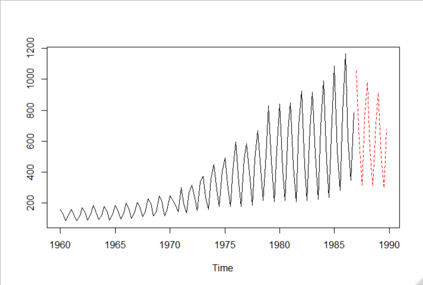
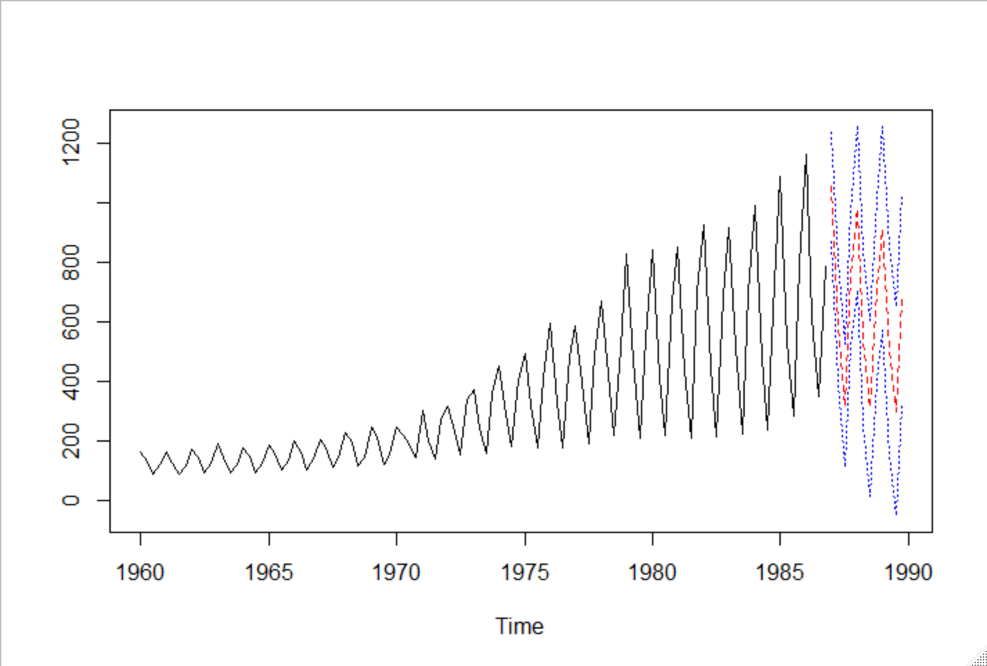
95%区間

結果はいまいち


ar(UKgas)

Call:
ar(x = UKgas)

Coefficients:
      1        2        3        4        5        6  
 0.5284  -0.2951   0.5844   0.3489   0.0436  -0.2709  

Order selected 6  sigma^2 estimated as  8496


#独立性の検定　Box-Pierce検定　Ljung-Box検定
Box.test(ar.UKgas$res, type = "Ljung")

Box-Ljung test

data:  ar.UKgas$res
X-squared = 2.2024, df = 1, p-value = 0.1378

# 正規性検定　ジャック・ベラ検定
ar.UKgas$res[-(1:6)]%>%
  jarque.bera.test()

Jarque Bera Test

data:  .
X-squared = 19.1, df = 2, p-value = 7.122e-05

#予測　12　四半期　3年先まで予測
UKgas.pred <- predict(ar.UKgas, n.ahead = 12)

$pred
          Qtr1      Qtr2      Qtr3      Qtr4
1987 1053.9970  600.7282  316.9538  748.8121
1988  981.4623  546.8309  308.6325  708.0975
1989  912.3671  504.7132  297.3734  674.2334

$se
          Qtr1      Qtr2      Qtr3      Qtr4
1987  92.17482 104.24961 104.25994 111.21667
1988 137.88835 147.29676 147.31935 151.18307
1989 170.10928 175.66459 175.66783 178.40438

ts.plot(UKgas,UKgas.pred$pred,
        gpars=list(lt=c(1,2),col=c(1,2)))

# 　95%区間（±2σ）でプロット
SE1<-UKgas.pred$pred+2*UKgas.pred$se
SE2<-UKgas.pred$pred-2*UKgas.pred$se
ts.plot(UKgas,UKgas.pred$pred,
        SE1,SE2,gpars=list(lt=c(1,2,3,3),col=c(1,2,4,4)))

差分を対数にしてでARモデルを試す

独立性がありそう、相関関係がなさそう
正規性は変わらずありそう（なさそうじゃないかな？）

プロット省略


UKgas_log_diff <- UKgas %>% log() %>% diff()
ar.UKgas_log_diff <- ar(UKgas_log_diff)

#独立性検定
Box.test(ar.UKgas_log_diff$res, type = "Ljung")

Box-Ljung test

data:  ar.UKgas_log_diff$res
X-squared = 7.0796, df = 1, p-value = 0.007797

#正規性検定
ar.UKgas_log_diff$res[-(1:3)]%>%
  jarque.bera.test()

Jarque Bera Test

data:  .
X-squared = 163.92, df = 2, p-value < 2.2e-16

#予測
UKgas_log_diff.pred

$pred
           Qtr1       Qtr2       Qtr3       Qtr4
1987  0.4464858 -0.6393982 -0.5191298  0.7510022
1988  0.4517140 -0.6265824 -0.4823045  0.7013768
1989  0.4485959 -0.6073688 -0.4532143  0.6595974

$se
          Qtr1      Qtr2      Qtr3      Qtr4
1987 0.1548956 0.2068423 0.2089726 0.2105422
1988 0.2449782 0.2685604 0.2726472 0.2756092
1989 0.2951754 0.3091888 0.3143251 0.3179931

# diffをcumsumで元に戻して、expすると予測値が得られる

Pythonで頑張ってみる

RからUKgasをcsv出力
pandasでcsvを読み込むが、index (date、Qt1,Qt2,,)が抜けていたので
indexを追加
　（Rから出力する際に、write.tableのrow.names=Tにしてみたけどダメだった、、？）
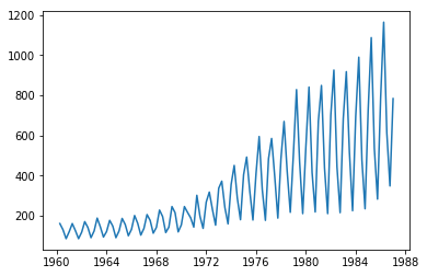
プロット　読み込みOK



#RでUKgasをcsv出力
write.table(UKgas, "UKgas2.csv", sep=",", row.names=T)

#Pythonのpandasで読み込み

import pandas as pd
import numpy as np
import matplotlib.pyplot as plt

UKgas = pd.read_csv('UKgas.csv')
UKgas['date']=pd.date_range('1960','1987',freq='Q')
UKgas.set_index('date', inplace=True)

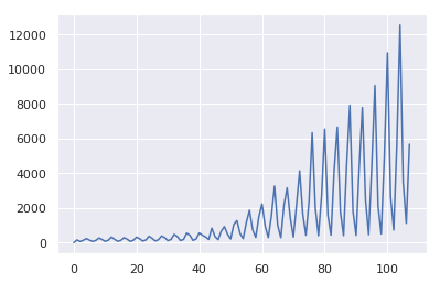
#プロットしてみる
plt.plot(UKgas)

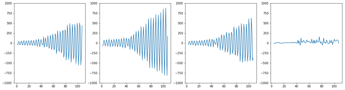
①差分データをプロットしてみる

差分データを作って引くか　.shift()
差分データをそのまま作るか　.diff() どちらも可能

4半期データなので差分1～4でプロット


plt.figure(figsize=(20,5))

plt.subplot(1,4,1)
plt.plot(UKgas - UKgas.shift(1))
#plt.plot(UKgas.diff())
plt.ylim(-1000,1000)

plt.subplot(1,4,2)
plt.plot(UKgas - UKgas.shift(2))
plt.ylim(-1000,1000)

plt.subplot(1,4,3)
plt.plot(UKgas - UKgas.shift(3))
plt.ylim(-1000,1000)

plt.subplot(1,4,4)
plt.plot(UKgas - UKgas.shift(4))
plt.ylim(-1000,1000)

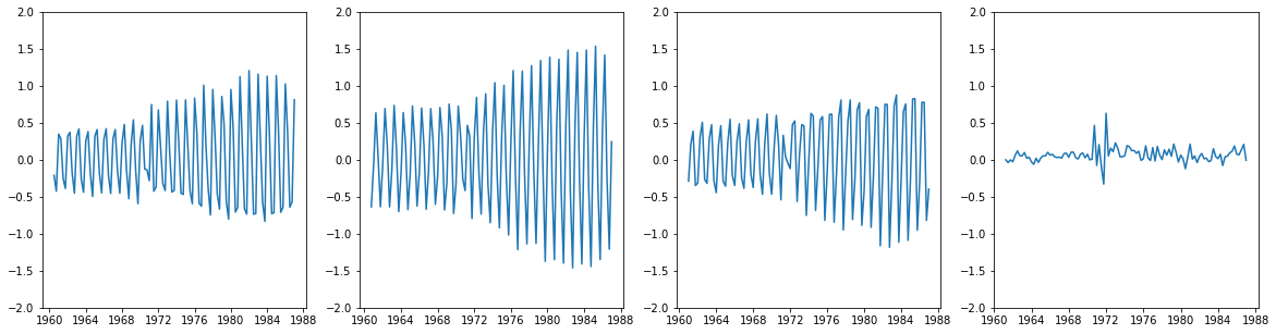
②対数にしてみる


plt.figure(figsize=(20,5))

plt.subplot(1,4,1)
plt.plot(np.log(UKgas).diff(1))
plt.ylim(-2,2)

plt.subplot(1,4,2)
plt.plot(np.log(UKgas).diff(2))
plt.ylim(-2,2)

plt.subplot(1,4,3)
plt.plot(np.log(UKgas).diff(3))
plt.ylim(-2,2)

plt.subplot(1,4,4)
plt.plot(np.log(UKgas).diff(4))
plt.ylim(-2,2)

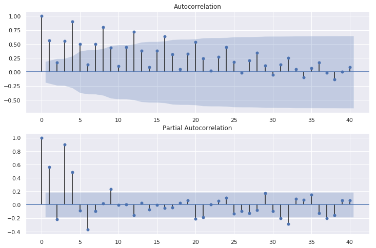
③自己相関関数（acf:autocorrelation function)で周期性を見てみる

重回帰と同じライブラリーstatsmodelsで自己相関関数を利用することができる
プロットも同じライブラリーで描画可能
matplotlibでplotしてしまうと折れ線グラフになりみにくい、、Rは適時切り替えてくれて便利、、
barとも違うし、このグラフはなんていうグラフなんでしょうか？

結果は同じように、4半期周期で相関がみられますね
偏自己相関をとると1年後の相関が強いことがわかります

グラフの網かけは95%区間です、これは便利


import statsmodels.api as sm

#自己相関を求める
# nlag のデフォルトは40  ラグ0～40までの41個の自己相関係数を出力　0は自分自身なので常に1

UKgas_acf = sm.tsa.stattools.acf(UKgas ,nlags = 40)
UKgas_acf

array([ 1.        ,  0.55962589,  0.16543426,  0.5579524 ,  0.90152719,
        0.49563309,  0.13309608,  0.49676976,  0.80555787,  0.434424  ,
        0.10824271,  0.44067708,  0.71960196,  0.37821433,  0.08281566,
        0.37936599,  0.63341685,  0.31724604,  0.0517523 ,  0.32556113,
        0.53930818,  0.24440861,  0.0192022 ,  0.26542743,  0.44460168,
        0.17427765, -0.01797088,  0.20634612,  0.34597344,  0.11226117,
       -0.05301067,  0.13370736,  0.24803597,  0.04672887, -0.09449297,
        0.06384167,  0.16578529, -0.01332281, -0.13163598,  0.00430394,
        0.08985417])

#  自己相関のグラフ      自己相関関数（ACF: autocorrelation function）
# StatsModelsのgraphics.tsa.plot_acf() で計算とプロットを同時にできる
# 偏自己相関（PACF:Pertial Autocorrelation Function）

fig = plt.figure(figsize=(12,8))
ax1 = fig.add_subplot(211)
fig = sm.graphics.tsa.plot_acf(UKgas, lags=40, ax=ax1)
ax2 = fig.add_subplot(212)
fig = sm.graphics.tsa.plot_pacf(UKgas, lags=40, ax=ax2)

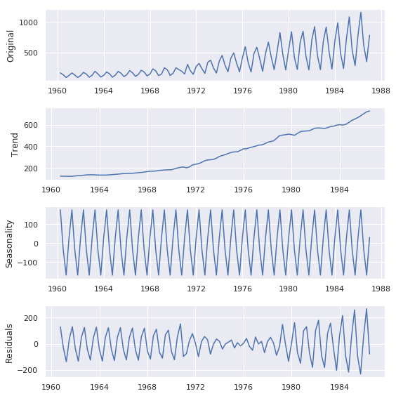
stastmodelsのseasonal_decomposeを使うと、トレンド、季節性、残差を確認できる


# statsmodel のseasonal_decomposeで俯瞰データ出力　　　オリジナル、トレンド、季節性、残差

res = sm.tsa.seasonal_decompose(UKgas)

# res = sm.tsa.seasonal_decompose(passengers) # 解析結果は取得済み

original = UKgas # オリジナルデータ
trend = res.trend # トレンドデータ
seasonal = res.seasonal # 季節性データ
residual = res.resid # 残差データ

plt.figure(figsize=(8, 8)) # グラフ描画枠作成、サイズ指定

# オリジナルデータのプロット
plt.subplot(411) # グラフ4行1列の1番目の位置（一番上）
plt.plot(UKgas)
plt.ylabel('Original')

# trend データのプロット
plt.subplot(412) # グラフ4行1列の2番目の位置
plt.plot(trend)
plt.ylabel('Trend')

# seasonalデータ のプロット
plt.subplot(413) # グラフ4行1列の3番目の位置
plt.plot(seasonal)
plt.ylabel('Seasonality')

# residual データのプロット
plt.subplot(414) # グラフ4行1列の4番目の位置（一番下）
plt.plot(residual)
plt.ylabel('Residuals')

plt.tight_layout() # グラフの間隔を自動調整

④スペクトル分析をしてみる

statsモデルにピリオドグラムがあるので試してみる、、
あれ？予想と違う、、
パワースペクトル自体はFFTとかで出せそうですが、、periodogramの使い方確認します


from statsmodels.tsa.stattools import periodogram

UKgas_sp = periodogram(UKgas)

plt.plot(UKgas_sp)

⑤単位根検定をしてみる

wikiによると単位根検定は以下のようなものがある
太字がRで検証してみた検定
・拡張ディッキー–フラー検定
・ディッキー–フラー検定
・フィリップス–ペロン検定
・KPSS検定（英語版）
・Zivot–Andrews検定（英語版）

statsmodelsにadf検定は搭載されているのですが、、エラーが、、調査中です
検索してもRの情報が多いですね、、この辺がRの強いところかな

⑥ARモデル（自己回帰モデル）を見てみる

statsmodelsにARが入っています、そのままですがPythonの統計関係はstatsmodelsにほぼ入っていますね～
公式サイトの確認必要ですね、、
https://www.statsmodels.org/stable/index.html

モデルを学習して予測してみます
maxlagを2（周期以下）にするとうまく予測できていない、、初期から後半のバイアスがかかっているようですね

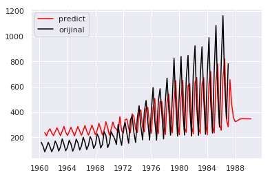
maxlagを4にするとそれなりに、、Rでの予測はあまりよくありませんでしたが、、
4以上では、パッと見た感じでは同程度でした


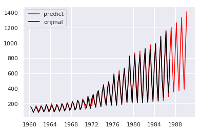
from statsmodels.tsa.ar_model import AR
%matplotlib inline
ar = AR(UKgas).fit(maxlag=4,ic='aic')
#予測
ar_predict = ar.predict(end=120)

#プロット
plt.plot(ar_predict,c='red',label="predict")
plt.plot(UKgas,c='black',label='orijinal')
plt.legend()
plt.show()

　　独立性検定　Box-Pierce検定をしてみる
　　正規性検定　Ljung-Box検定をしてみる
　
検定関係のいい関数がpythonで見つけられませんでした
実装しているひとは、ちらほらいるんですが、少し主旨とはずれるので、、
見つけたら追記します
事前調査はRで、実装はpythonってパターンが多いんですかね？

⑧差分を対数にしてARモデルを試す

検定した結果diffをが良好としているのですが、検定できていないので、、
diffデータを使うだけれであれば⑦と同じです

⑨ARMAモデル（自己回帰移動平均モデル）を試してみる

MA　移動平均モデルとARの二つを足したモデル
使用するにあたっては、ARとMRの次数を決める必要があります

aicが最小になる、AR　3,MA 2の組み合わせがいい感じ
この先でうまく予想ができない、、予測値がすべてNaNに、、調べて追記します


from statsmodels.tsa import stattools as st

# ARMAモデルの次数を決める
st.arma_order_select_ic(UKgas, ic='aic', trend = 'nc')

{'aic':              0            1            2
 0          NaN  1495.582257  1435.927808
 1  1479.809575  1448.623957  1424.508152
 2  1481.530412  1438.384552  1388.008218
 3  1208.282570  1152.034673  1118.209335
 4          NaN  1122.133937  1172.926357, 'aic_min_order': (3, 2)}

#ARMA予測 
from statsmodels.tsa.arima_model import ARMA
arma_UKgas = ARMA(UKgas,order=[3,2]).fit(maxlags=2, ic='aic')
arma_UKgas_predict = arma_UKgas.predict(end=120)
plt.plot(arma_UKgas_predict)

以下も追記予定、、

統計関係はRのほうが充実していることが身に染みてわかりました、、、

⑧ARIMAモデル（自己回帰和分移動平均モデル）
⑨SARIMAモデル（季節的自己回帰和分移動平均モデル

RとPythonで時系列データ解析

はじめに

環境

何するの？

Rのコード

①差分データをプロット

②対数でプロット

③自己相関関数で周期性を見てみる

④スペクトル分析をしてみる

⑤単位根検定をしてみる

⑥ARモデル（自己回帰モデル）を見てみる

差分を対数にしてでARモデルを試す

Pythonで頑張ってみる

①差分データをプロットしてみる

②対数にしてみる

③自己相関関数（acf:autocorrelation function)で周期性を見てみる

④スペクトル分析をしてみる

⑤単位根検定をしてみる

⑥ARモデル（自己回帰モデル）を見てみる

⑧差分を対数にしてARモデルを試す

⑨ARMAモデル（自己回帰移動平均モデル）を試してみる

以下も追記予定、、