はじめに
R未経験にもかかわらずR対象のデータ分析系の勉強会に出席してしまったので
Pythonだとどうするの?を復習を兼ねて記録に残したいと思います
改訂2
PythonでもRのように、目的変数と説明変数を指定することができました
備忘録として追記しました
改訂
勉強会参加メンバーから疑問点について助言いただいたので文末に追記しました
python で決定係数を出力した際、scikit learnとstatsmodelsに差がありました
statsmodelsの設定により差が発生していたことがわかりました
statsmodelsのデフォルトは、切片0とのこと
A intercept is not included by default and should be added by the user.
See statsmodels.tool.add_constant.
↓公式documents
https://www.statsmodels.org/dev/generated/statsmodels.regression.linear_model.OLS.html
別件でscikit-learnの intercept = False も結果がおかしくなるとの噂も、、、
この辺は別にまとめたいと思っています
環境
windows10 Pro 64bit
R :3.6.1
RStudio :1.2.1335
Google Colaboratoryを使用
Python :3.6.8
何するの?
RのSMCRM内のcustomerAcquisitionデータセットを利用して重回帰分析を行う
library(SMCRM)

# データセットの読み出し
data("customerAcquisition")

# データセットの確認
str(customerAcquisition)

'data.frame':	500 obs. of  16 variables:
 $ customer      : num  1 2 3 4 5 6 7 8 9 10 ...
 $ acquisition   : num  1 0 0 1 1 0 0 0 1 1 ...
 $ first_purchase: num  434 0 0 226 363 ...
 $ clv           : num  0 0 0 5.73 0 ...
 $ duration      : num  384 0 0 730 579 0 0 0 730 730 ...
 $ censor        : num  0 0 0 1 0 0 0 0 1 1 ...
 $ acq_expense   : num  760 148 253 610 672 ...
 $ acq_expense_sq: num  578147 21815 63787 371771 452068 ...
 $ industry      : num  1 1 1 1 1 0 0 0 1 1 ...
 $ revenue       : num  30.2 39.8 54.9 45.8 69 ...
 $ employees     : num  1240 166 1016 122 313 ...
 $ ret_expense   : num  2310 0 0 2193 801 ...
 $ ret_expense_sq: num  5335130 0 0 4807451 641825 ...
 $ crossbuy      : num  5 0 0 2 4 0 0 0 1 1 ...
 $ frequency     : num  2 0 0 12 7 0 0 0 11 14 ...
 $ frequency_sq  : num  4 0 0 144 49 0 0 0 121 196 ...

# acquisition が 1のデータを対象としてdf に代入
df<- customerAcquisition %>% filter(acquisition == 1)

# first_purchase を目的関数、その他すべてのデータを説明関数として重回帰
lm_CA_full <- lm(first_purchase ~ . - acquisition , data = df)

# first_purchase を目的関数、説明関数を4つに絞って重回帰
lm_CA <- lm(first_purchase ~ acq_expense + acq_expense_sq + revenue + employees, data = df)

# lm_CAの回帰計算結果表示
summary(lm_CA)

Call:
lm(formula = first_purchase ~ acq_expense + acq_expense_sq +
    revenue + employees, data = df)

Residuals:
    Min      1Q  Median      3Q     Max
-84.734 -19.765  -0.867  19.986 100.291

Coefficients:
                 Estimate Std. Error t value Pr(>|t|)
(Intercept)     7.783e+00  3.150e+01   0.247    0.805
acq_expense     5.317e-01  9.534e-02   5.577 5.66e-08 ***
acq_expense_sq -6.544e-04  7.192e-05  -9.099  < 2e-16 ***
revenue         2.986e+00  1.086e-01  27.488  < 2e-16 ***
employees       2.483e-01  3.769e-03  65.887  < 2e-16 ***
---
Signif. codes:  0 ‘***’ 0.001 ‘**’ 0.01 ‘*’ 0.05 ‘.’ 0.1 ‘ ’ 1

Residual standard error: 30.59 on 287 degrees of freedom
Multiple R-squared:  0.9617,	Adjusted R-squared:  0.9611
F-statistic:  1800 on 4 and 287 DF,  p-value: < 2.2e-16
説明係数の回帰係数は以下
acq_expense 5.317e-01
acq_expense_sq -6.544e-04
revenue 2.986e+00
employees 2.483e-01
切片は
(Intercept) 7.783e+00
線形回帰モデルは以下で表せる
first_purchase = 7.783e+00
+ acq_expense x 5.317e-01
+ acq_expense_sq x -6.544e-04
+ revenue x 2.986e+00
+ employees x 2.483e-01
モデルの評価値は決定係数で表される
決定係数 Multiple R-squared: 0.9617
修正決定係数 Adjusted R-squared: 0.9611
モデル同士の比較はAIC(赤池情報量基準)にて評価
> # AICで比較
> AIC(lm_CA_full)
[1] 2842.858
> AIC(lm_CA)
[1] 2833.373
AICの値が小さいほうが理想に近いということらしいので、すべての説明変数を利用したモデルより
4つの説明変数のモデルのほうがよく説明できているモデルということになる。
ではこれがベストか?はstepAICで調べられる。(らしい、、)
> lm_CA_step <- stepAIC(lm_CA_full)
Start:  AIC=2012.2
first_purchase ~ (customer + acquisition + clv + duration + censor +
    acq_expense + acq_expense_sq + industry + revenue + employees +
    ret_expense + ret_expense_sq + crossbuy + frequency + frequency_sq) -
    acquisition

                 Df Sum of Sq     RSS    AIC
- customer        1       238  259372 2010.5
- crossbuy        1       259  259394 2010.5
- duration        1       555  259690 2010.8
- frequency_sq    1       621  259756 2010.9
- ret_expense_sq  1       712  259847 2011.0
- ret_expense     1      1414  260549 2011.8
<none>                         259135 2012.2
- frequency       1      2075  261210 2012.5
- censor          1      2283  261418 2012.8
- clv             1      3111  262246 2013.7
- industry        1      3131  262266 2013.7
- acq_expense     1     23542  282677 2035.6
- acq_expense_sq  1     47453  306588 2059.3
- revenue         1    536393  795528 2337.7
- employees       1   3231713 3490848 2769.6

Step:  AIC=2010.47
first_purchase ~ clv + duration + censor + acq_expense + acq_expense_sq +
    industry + revenue + employees + ret_expense + ret_expense_sq +
    crossbuy + frequency + frequency_sq

                 Df Sum of Sq     RSS    AIC
- crossbuy        1       213  259586 2008.7
- duration        1       536  259909 2009.1
- frequency_sq    1       568  259941 2009.1
- ret_expense_sq  1       737  260109 2009.3
- ret_expense     1      1448  260820 2010.1
<none>                         259372 2010.5
- frequency       1      1981  261354 2010.7
- censor          1      2200  261573 2010.9
- industry        1      3009  262381 2011.8
- clv             1      3038  262411 2011.9
- acq_expense     1     23644  283017 2033.9
- acq_expense_sq  1     47614  306987 2057.7
- revenue         1    538374  797746 2336.5
- employees       1   3277066 3536439 2771.3

Step:  AIC=2008.71
first_purchase ~ clv + duration + censor + acq_expense + acq_expense_sq +
    industry + revenue + employees + ret_expense + ret_expense_sq +
    frequency + frequency_sq

                 Df Sum of Sq     RSS    AIC
- duration        1       394  259980 2007.2
- frequency_sq    1       496  260082 2007.3
- ret_expense_sq  1       812  260398 2007.6
- ret_expense     1      1428  261014 2008.3
<none>                         259586 2008.7
- frequency       1      1803  261388 2008.7
- censor          1      2000  261586 2009.0
- industry        1      2810  262396 2009.8
- clv             1      2890  262475 2009.9
- acq_expense     1     24239  283825 2032.8
- acq_expense_sq  1     50080  309666 2058.2
- revenue         1    554513  814098 2340.5
- employees       1   3297327 3556912 2771.0

Step:  AIC=2007.15
first_purchase ~ clv + censor + acq_expense + acq_expense_sq +
    industry + revenue + employees + ret_expense + ret_expense_sq +
    frequency + frequency_sq

                 Df Sum of Sq     RSS    AIC
- frequency_sq    1       495  260474 2005.7
- ret_expense_sq  1       605  260585 2005.8
- ret_expense     1      1068  261048 2006.3
- censor          1      1606  261586 2007.0
- frequency       1      1609  261589 2007.0
<none>                         259980 2007.2
- industry        1      2419  262399 2007.8
- clv             1      2502  262481 2007.9
- acq_expense     1     31416  291395 2038.5
- acq_expense_sq  1     77789  337769 2081.6
- revenue         1    594439  854419 2352.6
- employees       1   3327401 3587380 2771.5

Step:  AIC=2005.7
first_purchase ~ clv + censor + acq_expense + acq_expense_sq +
    industry + revenue + employees + ret_expense + ret_expense_sq +
    frequency

                 Df Sum of Sq     RSS    AIC
- ret_expense_sq  1       651  261125 2004.4
- ret_expense     1      1052  261527 2004.9
- censor          1      1382  261856 2005.2
<none>                         260474 2005.7
- clv             1      2202  262677 2006.2
- industry        1      2341  262815 2006.3
- frequency       1      5221  265695 2009.5
- acq_expense     1     31388  291862 2036.9
- acq_expense_sq  1     77902  338376 2080.1
- revenue         1    612592  873066 2356.9
- employees       1   3335399 3595873 2770.2

Step:  AIC=2004.43
first_purchase ~ clv + censor + acq_expense + acq_expense_sq +
    industry + revenue + employees + ret_expense + frequency

                 Df Sum of Sq     RSS    AIC
- ret_expense     1       796  261921 2003.3
- censor          1      1429  262554 2004.0
<none>                         261125 2004.4
- clv             1      2225  263349 2004.9
- industry        1      2402  263527 2005.1
- frequency       1      5500  266625 2008.5
- acq_expense     1     30890  292015 2035.1
- acq_expense_sq  1     77273  338398 2078.1
- revenue         1    621020  882145 2357.9
- employees       1   3347586 3608711 2769.3

Step:  AIC=2003.32
first_purchase ~ clv + censor + acq_expense + acq_expense_sq +
    industry + revenue + employees + frequency

                 Df Sum of Sq     RSS    AIC
- censor          1       929  262850 2002.3
- clv             1      1489  263410 2003.0
<none>                         261921 2003.3
- industry        1      2086  264008 2003.6
- frequency       1      4822  266743 2006.7
- acq_expense     1     30126  292047 2033.1
- acq_expense_sq  1     76673  338594 2076.3
- revenue         1    674215  936136 2373.2
- employees       1   3509176 3771097 2780.1

Step:  AIC=2002.35
first_purchase ~ clv + acq_expense + acq_expense_sq + industry +
    revenue + employees + frequency

                 Df Sum of Sq     RSS    AIC
- clv             1      1250  264100 2001.7
<none>                         262850 2002.3
- industry        1      1902  264752 2002.5
- frequency       1      4941  267791 2005.8
- acq_expense     1     29200  292049 2031.1
- acq_expense_sq  1     76005  338855 2074.5
- revenue         1    679663  942512 2373.2
- employees       1   3892379 4155229 2806.4

Step:  AIC=2001.74
first_purchase ~ acq_expense + acq_expense_sq + industry + revenue +
    employees + frequency

                 Df Sum of Sq     RSS    AIC
- industry        1      1233  265333 2001.1
<none>                         264100 2001.7
- frequency       1      3738  267838 2003.8
- acq_expense     1     28352  292452 2029.5
- acq_expense_sq  1     76467  340567 2074.0
- revenue         1    693588  957688 2375.9
- employees       1   3962665 4226765 2809.4

Step:  AIC=2001.1
first_purchase ~ acq_expense + acq_expense_sq + revenue + employees +
    frequency

                 Df Sum of Sq     RSS    AIC
<none>                         265333 2001.1
- frequency       1      3303  268636 2002.7
- acq_expense     1     28868  294201 2029.3
- acq_expense_sq  1     77127  342460 2073.6
- revenue         1    706100  971433 2378.1
- employees       1   3973948 4239281 2808.3
StartのAICが2012.2で単独で評価した2842.858となぜ異なるのかわかりませんが、ベストなモデルは
初めに選択した4つの説明変数に、frequencyを追加したものということが分かりました。
Pythonで記述
customerAcquisitionデータセットはPythonには用意されていないので、Rからcsvで出力して利用することにします
#RからcustomerAcquisitionをcsvで出力
write.table(customerAcquisition, "customerAcquisition.csv", sep=",", row.names=F)
Pythonでのデータ解析はライブラリーに依存しているところが多々あるため下記のようなライブラリーをインポートする必要がある
pandas データ分析用ライブラリ。DataFrameを提供
numpy 多次元配列計算用ライブラリ
matplotlib グラフ描画ライブラリ
seaborn matplotlibのラッパー、かっこいいグラフが簡単に書ける
sklearn 機械学習用ライブラリー
import numpy as np
import pandas as pd

# 可視化モジュール
import matplotlib.pyplot as plt
import seaborn as sns
sns.set()
%matplotlib inline

# 重回帰
from sklearn.linear_model import LinearRegression
Rから出力したcsvファイルはpandasで読み込み、データ構造も簡単に確認できます
df = pd.read_csv('customerAcquisition.csv')
df.info()

<class 'pandas.core.frame.DataFrame'>
RangeIndex: 500 entries, 0 to 499
Data columns (total 16 columns):
customer          500 non-null int64
acquisition       500 non-null int64
first_purchase    500 non-null float64
clv               500 non-null float64
duration          500 non-null int64
censor            500 non-null int64
acq_expense       500 non-null float64
acq_expense_sq    500 non-null float64
industry          500 non-null int64
revenue           500 non-null float64
employees         500 non-null int64
ret_expense       500 non-null float64
ret_expense_sq    500 non-null float64
crossbuy          500 non-null int64
frequency         500 non-null int64
frequency_sq      500 non-null int64
dtypes: float64(7), int64(9)
memory usage: 62.6 KB
データフレームは論理式でbool値を取得し、bool値を使ってデータを抽出することができる
df['acquisition'] == 1

0       True
1      False
2      False
3       True
  ...
497    False
498     True
499    False
Name: acquisition, Length: 500, dtype: bool

# acquisition が 1 のデータのみに抽出
df = df[df['acquisition'] == 1]

# 抽出後のデータを確認
df.info()

<class 'pandas.core.frame.DataFrame'>
Int64Index: 292 entries, 0 to 498
Data columns (total 16 columns):
customer          292 non-null int64
acquisition       292 non-null int64
first_purchase    292 non-null float64
clv               292 non-null float64
duration          292 non-null int64
censor            292 non-null int64
acq_expense       292 non-null float64
acq_expense_sq    292 non-null float64
industry          292 non-null int64
revenue           292 non-null float64
employees         292 non-null int64
ret_expense       292 non-null float64
ret_expense_sq    292 non-null float64
crossbuy          292 non-null int64
frequency         292 non-null int64
frequency_sq      292 non-null int64
dtypes: float64(7), int64(9)
memory usage: 38.8 KB
acquisition = 1 のみのデータ抽出でデータ数が
500 → 292 に減少
このデータフレームをベースに目的変数、説明変数を作りながら
重回帰のclassにデータを入れていきます
# 目的変数
y = df['first_purchase']

# 説明変数は元のデータフレームから目的変数を削除したもの
X_full = df.drop('first_purchase',axis=1)

# 選択した説明変数のデータフレームも作成
df_sel = df[['first_purchase','acq_expense','acq_expense_sq','revenue','employees']]
X_sel = df_sel.drop('first_purchase',axis=1)

# 重回帰のインスタンスを作成
model = LinearRegression()

# X_selで学習
model.fit(X_sel,y)

# 回帰係数
print('\n回帰係数\n{}'.format(pd.Series(model.coef_, index=df_sel.drop('first_purchase',axis=1).columns)))

回帰係数
acq_expense       0.531689
acq_expense_sq   -0.000654
revenue           2.986234
employees         0.248334
dtype: float64

# 切片
print('切片: {:.3f}'.format(model.intercept_))

切片: 7.783

# 決定係数
print(model.score(df_sel.drop('first_purchase',axis=1),df_sel['first_purchase']))

0.962
回帰係数、切片ともにRと同様に求められたが
評価値は決定係数のみで修正決定係数は出力できない(と思う、、追記に記載しました)
Pythonの重回帰は機械学習モデルとしてLinearRegressionしか使ったことがなかったが、Rのように統計的な結出力を得たい場合は、statsmodelsで可能となるようです。
from sklearn import datasets
from statsmodels import api as sm

model = sm.OLS(y, X_sel)
result = model.fit()
print (result.summary())

                                 OLS Regression Results
=======================================================================================
Dep. Variable:         first_purchase   R-squared (uncentered):                   0.994
Model:                            OLS   Adj. R-squared (uncentered):              0.994
Method:                 Least Squares   F-statistic:                          1.266e+04
Date:                Tue, 13 Aug 2019   Prob (F-statistic):                   3.21e-322
Time:                        14:44:24   Log-Likelihood:                         -1410.7
No. Observations:                 292   AIC:                                      2829.
Df Residuals:                     288   BIC:                                      2844.
Df Model:                           4
Covariance Type:            nonrobust
==================================================================================
                     coef    std err          t      P>|t|      [0.025      0.975]
----------------------------------------------------------------------------------
acq_expense        0.5546      0.023     24.391      0.000       0.510       0.599
acq_expense_sq    -0.0007   2.42e-05    -27.743      0.000      -0.001      -0.001
revenue            2.9894      0.108     27.755      0.000       2.777       3.201
employees          0.2486      0.004     69.021      0.000       0.242       0.256
==============================================================================
Omnibus:                        2.317   Durbin-Watson:                   1.891
Prob(Omnibus):                  0.314   Jarque-Bera (JB):                2.013
Skew:                           0.156   Prob(JB):                        0.366
Kurtosis:                       3.260   Cond. No.                     2.97e+04
==============================================================================

Warnings:
[1] Standard Errors assume that the covariance matrix of the errors is correctly specified.
[2] The condition number is large, 2.97e+04. This might indicate that there are
strong multicollinearity or other numerical problems.


print(result.aic)

2829.4353329751475
修正決定係数まで出力できたが、、、結果が異なる、、
AICも微妙に違う、、なぜ?
Pythonでは、調べた限りではRのようなstepAICはなく自分で組む必要がありそう
Qiitaでも自作している人がちらほら
データが異なる理由、stepAICはじっくり調べてみたいと思います
とりあえず、Rとpythonで同じデータセットを用いて重回帰を行ってみました
Rは初めてでしたが、さすが統計的な扱いは得意ですね、楽そうなのでサクッと計算ができそうです
必要に応じて使い分けですかね?
Rでの勉強会はまだ続くのでpythonとの違いをじっくり調べてみたいと思います。
追記
scikit-learnとstatsmodelsの決定係数差について
statsmodelsで回帰を行う場合は、Xに明示的に切片(statsmodelssでhconstant)を追加する必要があった
デフォルトではなし
statsmodelsの結果
切片なしの決定係数 0.994
切片ありの决定係数 0.962
scikit-learnの結果
決定係数 0.962
Rの結果
決定係数 Multiple R-squared: 0.9617
修正決定係数 Adjusted R-squared: 0.9611
from sklearn import datasets
from statsmodels import api as sm

X_sel_ = sm.add_constant(X_sel)

model2 = sm.OLS(y, X_sel_)
result2 = model2.fit()
print (result2.summary())

                                                         OLS Regression Results
==============================================================================
Dep. Variable:         first_purchase   R-squared:                       0.962
Model:                            OLS   Adj. R-squared:                  0.961
Method:                 Least Squares   F-statistic:                     1800.
Date:                Sat, 31 Aug 2019   Prob (F-statistic):          7.74e-202
Time:                        03:58:27   Log-Likelihood:                -1410.7
No. Observations:                 292   AIC:                             2831.
Df Residuals:                     287   BIC:                             2850.
Df Model:                           4
Covariance Type:            nonrobust
==================================================================================
                     coef    std err          t      P>|t|      [0.025      0.975]
----------------------------------------------------------------------------------
const              7.7830     31.498      0.247      0.805     -54.213      69.779
acq_expense        0.5317      0.095      5.577      0.000       0.344       0.719
acq_expense_sq    -0.0007   7.19e-05     -9.099      0.000      -0.001      -0.001
revenue            2.9862      0.109     27.488      0.000       2.772       3.200
employees          0.2483      0.004     65.887      0.000       0.241       0.256
==============================================================================
Omnibus:                        2.045   Durbin-Watson:                   1.889
Prob(Omnibus):                  0.360   Jarque-Bera (JB):                1.739
Skew:                           0.150   Prob(JB):                        0.419
Kurtosis:                       3.230   Cond. No.                     8.58e+06
==============================================================================

Warnings:
[1] Standard Errors assume that the covariance matrix of the errors is correctly specified.
[2] The condition number is large, 8.58e+06. This might indicate that there are
strong multicollinearity or other numerical problems.


print(result2.aic)

2831.3732200478385
scikit-learnの自由度修正決定係数の扱いについて
scikit-learnでは決定係数のみのようです
自由度調整決定係数は決定係数から計算できるので試してみました
https://www.statisticshowto.datasciencecentral.com/adjusted-r2/
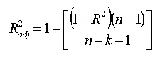
R,修正後のstatsmodelsとも数値が合いました!
# 調整決系係数
y= df_sel['first_purchase']
X_sel = df_sel.drop('first_purchase',axis=1).columns

adj_r_sqr = 1 - (1-r_sqr)*(len(y)-1)/(len(y)-len(X_sel)-1)

print('adj_r_sqr = :',adj_r_sqr)

adj_r_sqr = : 0.9611309093220055
追記2
statsmodels.formula.api を用いると、R-styleのモデル式が使用できます
statsmodels.formula.api: A convenience interface for specifying models using formula strings and DataFrames. This API directly exposes the from_formula class method of models that support the formula API. Canonically imported using import statsmodels.formula.api as smf
import statsmodels.formula.api as smf

model_Rlike = smf.ols('first_purchase ~ acq_expense + acq_expense_sq + revenue + employees', data=df_sel)
result = model_Rlike.fit()
print(result.summary())

                           OLS Regression Results
==============================================================================
Dep. Variable:         first_purchase   R-squared:                       0.962
Model:                            OLS   Adj. R-squared:                  0.961
Method:                 Least Squares   F-statistic:                     1800.
Date:                Sun, 03 May 2020   Prob (F-statistic):          7.74e-202
Time:                        10:19:15   Log-Likelihood:                -1410.7
No. Observations:                 292   AIC:                             2831.
Df Residuals:                     287   BIC:                             2850.
Df Model:                           4
Covariance Type:            nonrobust
==================================================================================
                     coef    std err          t      P>|t|      [0.025      0.975]
----------------------------------------------------------------------------------
Intercept          7.7830     31.498      0.247      0.805     -54.213      69.779
acq_expense        0.5317      0.095      5.577      0.000       0.344       0.719
acq_expense_sq    -0.0007   7.19e-05     -9.099      0.000      -0.001      -0.001
revenue            2.9862      0.109     27.488      0.000       2.772       3.200
employees          0.2483      0.004     65.887      0.000       0.241       0.256
==============================================================================
Omnibus:                        2.045   Durbin-Watson:                   1.889
Prob(Omnibus):                  0.360   Jarque-Bera (JB):                1.739
Skew:                           0.150   Prob(JB):                        0.419
Kurtosis:                       3.230   Cond. No.                     8.58e+06
==============================================================================

Warnings:
[1] Standard Errors assume that the covariance matrix of the errors is correctly specified.
[2] The condition number is large, 8.58e+06. This might indicate that there are
strong multicollinearity or other numerical problems.
'''