はじめに
またまたRの勉強会に参加しました
今回は、機械学習の分類です、これはpythonの得意分野!と思ってましたが
解析データはRのほうが簡単に詳細出せます
色々なモデルをサクッと試すのはpythonの方が楽そうですが、細かく解析するのはRの方が得意な気がします
目的は、Rの講習会の内容をpythonではどうやって書くの?を復習かねて記録しています
環境
windows10 Pro 64bit
R :3.6.1
RStudio :1.2.1335
Google Colaboratoryを使用
Python :3.6.8
何するの?
Rに組み込まれているデータセットVehicleを用いて分類モデルを作成する
①決定木でモデルを作成/評価
②モデルの可視化
③改良/評価
④可視化
⑤ランダムフォレストで実行/評価
Rのコード
データ準備
・読み込み
・データ確認
・トレーニングデータ、テストデータ分割
data(Vehicle)
str(Vehicle)

'data.frame':	846 obs. of  19 variables:
 $ Comp        : num  95 91 104 93 85 107 97 90 86 93 ...
 $ Circ        : num  48 41 50 41 44 57 43 43 34 44 ...
 $ D.Circ      : num  83 84 106 82 70 106 73 66 62 98 ...
 $ Rad.Ra      : num  178 141 209 159 205 172 173 157 140 197 ...
 $ Pr.Axis.Ra  : num  72 57 66 63 103 50 65 65 61 62 ...
 $ Max.L.Ra    : num  10 9 10 9 52 6 6 9 7 11 ...
 $ Scat.Ra     : num  162 149 207 144 149 255 153 137 122 183 ...
 $ Elong       : num  42 45 32 46 45 26 42 48 54 36 ...
 $ Pr.Axis.Rect: num  20 19 23 19 19 28 19 18 17 22 ...
 $ Max.L.Rect  : num  159 143 158 143 144 169 143 146 127 146 ...
 $ Sc.Var.Maxis: num  176 170 223 160 241 280 176 162 141 202 ...
 $ Sc.Var.maxis: num  379 330 635 309 325 957 361 281 223 505 ...
 $ Ra.Gyr      : num  184 158 220 127 188 264 172 164 112 152 ...
 $ Skew.Maxis  : num  70 72 73 63 127 85 66 67 64 64 ...
 $ Skew.maxis  : num  6 9 14 6 9 5 13 3 2 4 ...
 $ Kurt.maxis  : num  16 14 9 10 11 9 1 3 14 14 ...
 $ Kurt.Maxis  : num  187 189 188 199 180 181 200 193 200 195 ...
 $ Holl.Ra     : num  197 199 196 207 183 183 204 202 208 204 ...
 $ Class       : Factor w/ 4 levels "bus","opel","saab",..: 4 4 3 4 1 1 1 4 4 3 ...

set.seed(1234)
N <- nrow(Vehicle)
train_flg <- sample(1:N, 500, FALSE)
train  <- Vehicle[train_flg,]
test <- Vehicle[-train_flg,]

> NROW(train)
[1] 500
> NROW(test)
[1] 346
①決定木でモデルを作成/評価
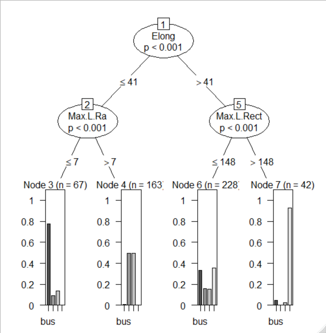
正解率は、0.4913
混合行列から、saabが予測できていないですね
fit <- ctree(Class ~., data = train,
             controls=ctree_control(maxdepth = 2))
fit

	 Conditional inference tree with 4 terminal nodes

Response:  Class
Inputs:  Comp, Circ, D.Circ, Rad.Ra, Pr.Axis.Ra, Max.L.Ra, Scat.Ra, Elong, Pr.Axis.Rect, Max.L.Rect, Sc.Var.Maxis, Sc.Var.maxis, Ra.Gyr, Skew.Maxis, Skew.maxis, Kurt.maxis, Kurt.Maxis, Holl.Ra
Number of observations:  500

1) Elong <= 41; criterion = 1, statistic = 149.268
  2) Max.L.Ra <= 7; criterion = 1, statistic = 139.722
    3)*  weights = 67
  2) Max.L.Ra > 7
    4)*  weights = 163
1) Elong > 41
  5) Max.L.Rect <= 148; criterion = 1, statistic = 67.057
    6)*  weights = 228
  5) Max.L.Rect > 148
    7)*  weights = 42

# 予測作成
pred_prob <- predict(fit, newdata=test, type="prob")
pred <- predict(fit, newdata=test, type="response")

# モデル評価
caret::confusionMatrix(pred, test$Class)

Confusion Matrix and Statistics

          Reference
Prediction bus opel saab van
      bus   34    3    3   0
      opel   0   57   55   0
      saab   0    0    0   0
      van   53   29   33  79

Overall Statistics

               Accuracy : 0.4913
                 95% CI : (0.4375, 0.5453)
    No Information Rate : 0.263
    P-Value [Acc > NIR] : < 2.2e-16

                  Kappa : 0.3304

 Mcnemar's Test P-Value : < 2.2e-16

Statistics by Class:

                     Class: bus Class: opel Class: saab Class: van
Sensitivity             0.39080      0.6404       0.000     1.0000
Specificity             0.97683      0.7860       1.000     0.5693
Pos Pred Value          0.85000      0.5089         NaN     0.4072
Neg Pred Value          0.82680      0.8632       0.737     1.0000
Prevalence              0.25145      0.2572       0.263     0.2283
Detection Rate          0.09827      0.1647       0.000     0.2283
Detection Prevalence    0.11561      0.3237       0.000     0.5607
Balanced Accuracy       0.68382      0.7132       0.500     0.7846
②モデルの可視化
plot(fit) だけで樹形図が出力できるのはいいですね
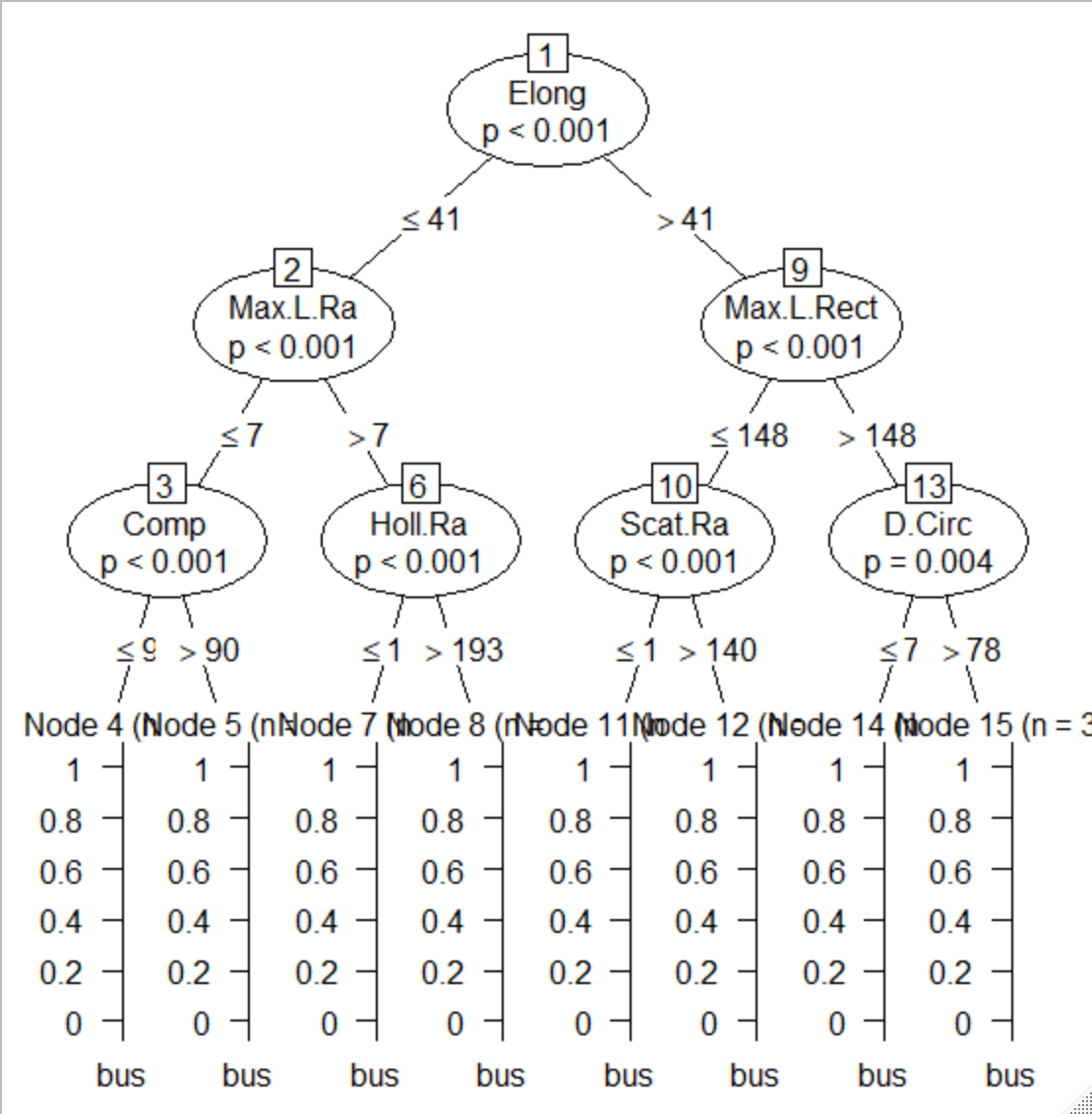
③改良/評価
階層を深くして改善
2層から3層へ深くして正解率が、0.4913から0.6069へ改善
saabの分類改善してますが、opelが改悪ですね、saabとopelはこの説明変数では難しそう
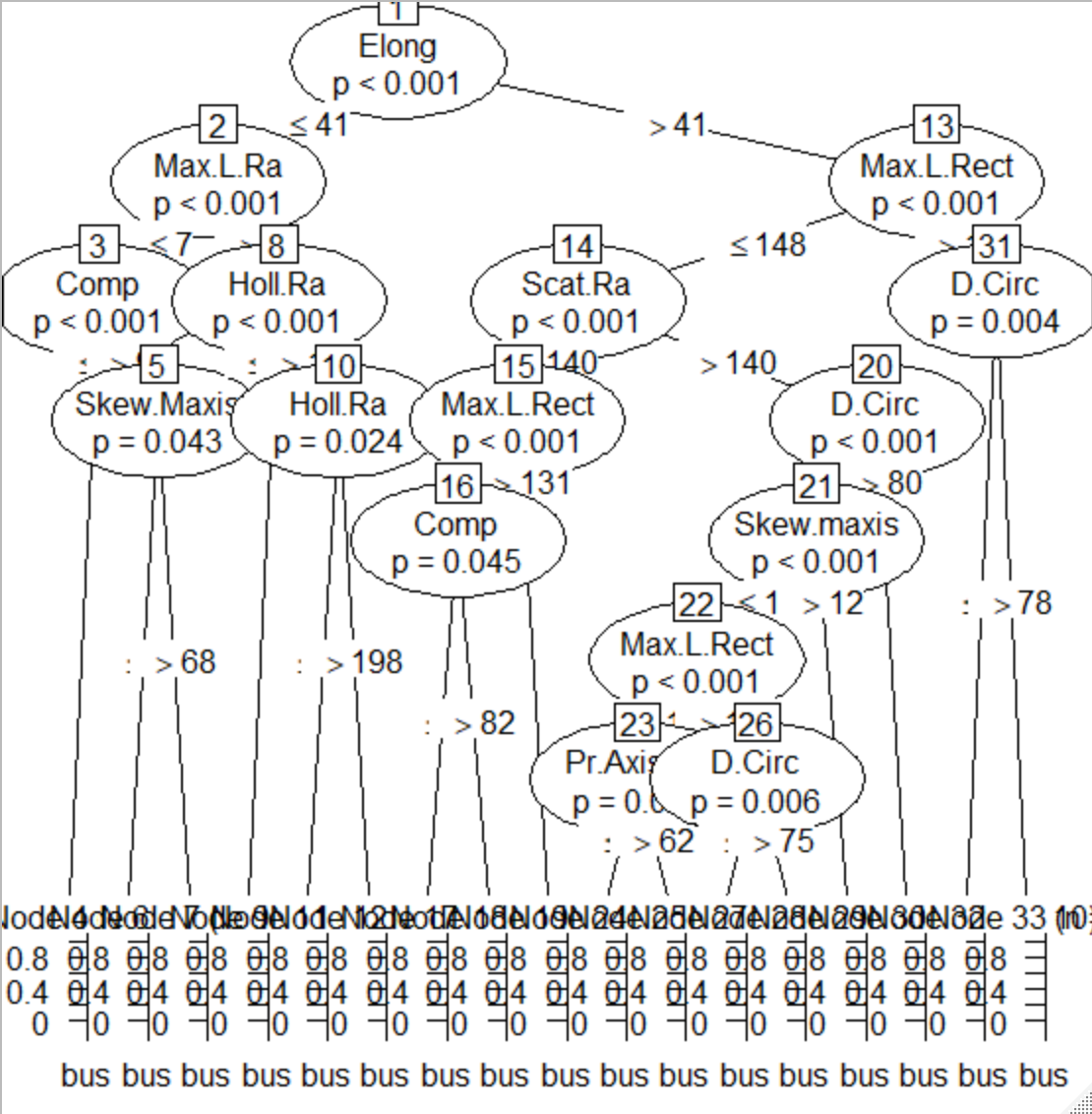
階層制限をなくしたモデルでは、正解率が0.6879まで向上
このモデルでも、saabとopelはうまく分類できていない
fit3 <- ctree(Class ~., data = train,
              controls=ctree_control(maxdepth = 3))
fitu <- ctree(Class ~., data = train)

pred3 <- predict(fit3, newdata=test, type="response")
predu <- predict(fitu, newdata=test, type="response")

# 階層3で評価
caret::confusionMatrix(pred3, test$Class)
Confusion Matrix and Statistics

          Reference
Prediction bus opel saab van
      bus   83   14   18  12
      opel   2    6    3   0
      saab   0   52   54   0
      van    2   17   16  67

Overall Statistics

               Accuracy : 0.6069
                 95% CI : (0.5533, 0.6587)
    No Information Rate : 0.263
    P-Value [Acc > NIR] : < 2.2e-16

                  Kappa : 0.4771

 Mcnemar's Test P-Value : < 2.2e-16

Statistics by Class:

                     Class: bus Class: opel Class: saab Class: van
Sensitivity              0.9540     0.06742      0.5934     0.8481
Specificity              0.8301     0.98054      0.7961     0.8689
Pos Pred Value           0.6535     0.54545      0.5094     0.6569
Neg Pred Value           0.9817     0.75224      0.8458     0.9508
Prevalence               0.2514     0.25723      0.2630     0.2283
Detection Rate           0.2399     0.01734      0.1561     0.1936
Detection Prevalence     0.3671     0.03179      0.3064     0.2948
Balanced Accuracy        0.8921     0.52398      0.6947     0.8585

# 制限なしで決定木モデルを作成
caret::confusionMatrix(predu, test$Class)
Confusion Matrix and Statistics

          Reference
Prediction bus opel saab van
      bus   80    4    6   6
      opel   3   41   25   1
      saab   2   29   45   0
      van    2   15   15  72

Overall Statistics

               Accuracy : 0.6879
                 95% CI : (0.6361, 0.7363)
    No Information Rate : 0.263
    P-Value [Acc > NIR] : < 2.2e-16

                  Kappa : 0.5848

 Mcnemar's Test P-Value : 1.872e-05

Statistics by Class:

                     Class: bus Class: opel Class: saab Class: van
Sensitivity              0.9195      0.4607      0.4945     0.9114
Specificity              0.9382      0.8872      0.8784     0.8801
Pos Pred Value           0.8333      0.5857      0.5921     0.6923
Neg Pred Value           0.9720      0.8261      0.8296     0.9711
Prevalence               0.2514      0.2572      0.2630     0.2283
Detection Rate           0.2312      0.1185      0.1301     0.2081
Detection Prevalence     0.2775      0.2023      0.2197     0.3006
Balanced Accuracy        0.9289      0.6739      0.6865     0.8958
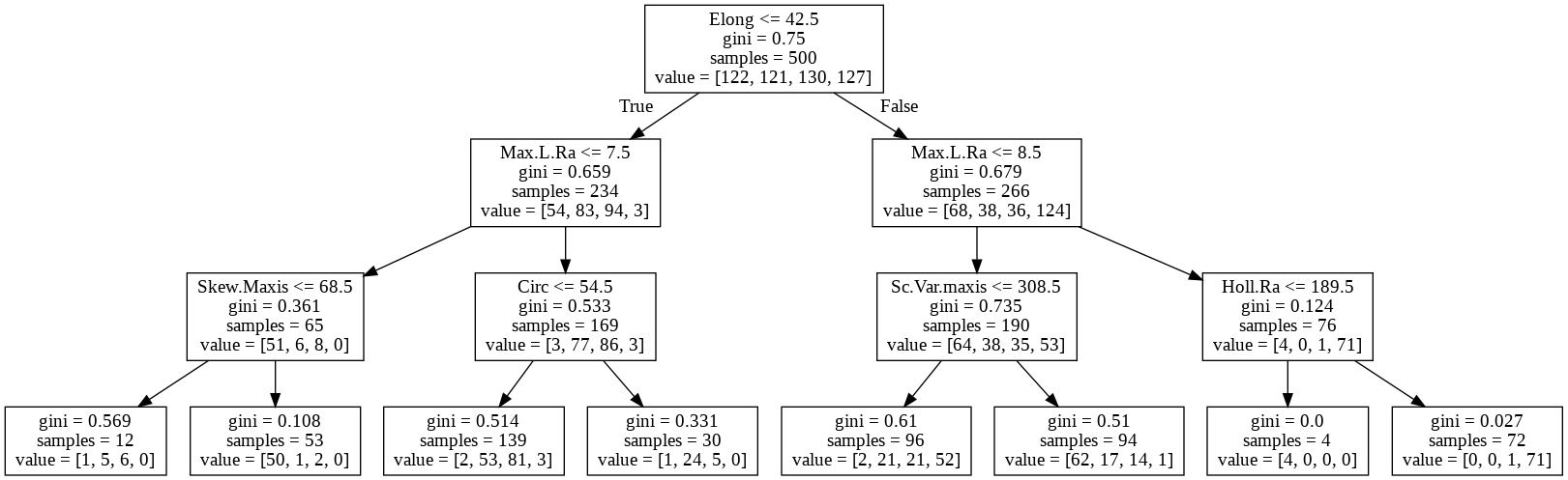
④可視化
3層モデルの樹形図
制限なしの樹形図
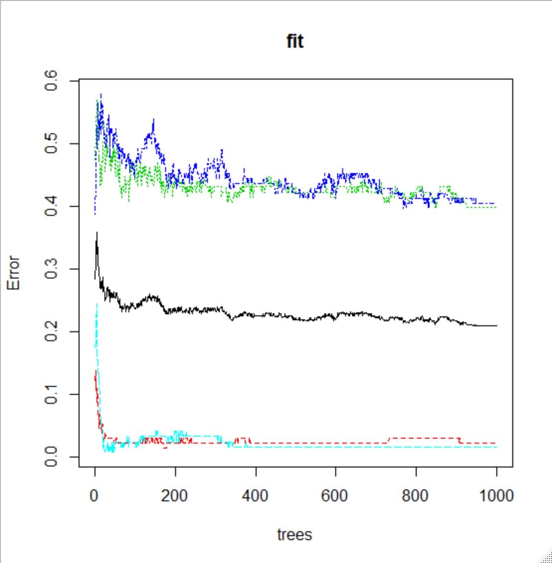
⑤ランダムフォレストで実行/評価
アンサンブル学習の一つである、ランダムフォレストを試してみる
モデルの説明が目的ではないのでざっくり説明ですが、ランダムフォレストは
決定木を何個も作り、結果の多数決で最終的な分類を行うようなモデル
試す決定木の数を num.tree で指定 今回は1000
正解率は、0.7312 で層を増やした決定木よりも良好
決定木の数とErrorの関係から、決定木を増やすとErrorが減る傾向にあることが確認できます
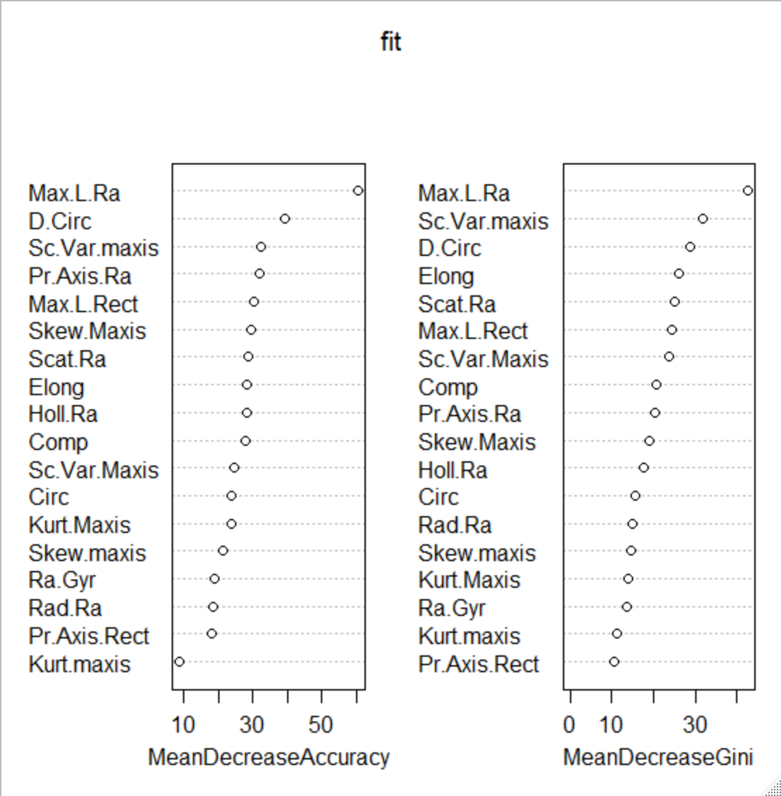
説明変数の重要度をvarImpPlotでグラフ化
まんべんなく使用されている
library(randomForest)
num.trees <- 1000
fit <- randomForest(Class ~ ., data = train, ntree = num.trees,
                    importance = TRUE, proximity = TRUE)
plot(fit)
varImpPlot(fit)
# 39.5_予測作成

pred <- predict(fit, test)
pred
caret::confusionMatrix(pred, test$Class)

Confusion Matrix and Statistics

          Reference
Prediction bus opel saab van
      bus   87    1    7   0
      opel   0   39   26   0
      saab   0   45   49   1
      van    0    4    9  78

Overall Statistics

               Accuracy : 0.7312
                 95% CI : (0.6812, 0.7772)
    No Information Rate : 0.263
    P-Value [Acc > NIR] : < 2.2e-16

                  Kappa : 0.6418

 Mcnemar's Test P-Value : NA

Statistics by Class:

                     Class: bus Class: opel Class: saab Class: van
Sensitivity              1.0000      0.4382      0.5385     0.9873
Specificity              0.9691      0.8988      0.8196     0.9513
Pos Pred Value           0.9158      0.6000      0.5158     0.8571
Neg Pred Value           1.0000      0.8221      0.8327     0.9961
Prevalence               0.2514      0.2572      0.2630     0.2283
Detection Rate           0.2514      0.1127      0.1416     0.2254
Detection Prevalence     0.2746      0.1879      0.2746     0.2630
Balanced Accuracy        0.9846      0.6685      0.6790     0.9693
pythonコード
pythonでデータフレームに読み込んで、ざっとデータを確認
カラムは19種類
Classのみ、object形式でその他は、数値データ
目的変数がclassなので説明変数はすべて数値データですね
データ数は、846個で欠損なし
データフレームのデータの確認には「pandas_profiling」が非常に優秀
情報量が多いので省きますが
総数、欠損値、ヒストグラム、相関係数等々 個別に実施しそうな項目を一気に表示してくれます
# RでVehicleをcsv出力
write.table(Vehicle, "Vehicle.csv", sep=",", row.names=T)


# いつものライブラリーでデータ入力
# ライブラリーは 標準>サードパーティ>ローカル で アルファベット順が基本とのことです
# 詳しくはPEP8などを参考に(今までめちゃくちゃでした、、)

import matplotlib.pyplot as plt
import numpy as np
import pandas as pd
import seaborn as sns

vehicle = pd.read_csv('Vehicle.csv')
vehicle.info()

<class 'pandas.core.frame.DataFrame'>
RangeIndex: 846 entries, 0 to 845
Data columns (total 19 columns):
Comp            846 non-null int64
Circ            846 non-null int64
D.Circ          846 non-null int64
Rad.Ra          846 non-null int64
Pr.Axis.Ra      846 non-null int64
Max.L.Ra        846 non-null int64
Scat.Ra         846 non-null int64
Elong           846 non-null int64
Pr.Axis.Rect    846 non-null int64
Max.L.Rect      846 non-null int64
Sc.Var.Maxis    846 non-null int64
Sc.Var.maxis    846 non-null int64
Ra.Gyr          846 non-null int64
Skew.Maxis      846 non-null int64
Skew.maxis      846 non-null int64
Kurt.maxis      846 non-null int64
Kurt.Maxis      846 non-null int64
Holl.Ra         846 non-null int64
Class           846 non-null object
dtypes: int64(18), object(1)
memory usage: 125.7+ KB
データフレームから目的変数と説明変数に分割
Rは別途作成しなくても目的変数が指定できるので便利
(scikit-learnもできるのでしょうか?)
データをトレーニングデータとテストデータに分割
train_test_splitはtestデータの割合、数の指定なので、846-500=346 指定
from sklearn.model_selection import train_test_split

train_y = vehicle['Class']
train_X = vehicle.drop('Class',axis = 1)

(train_X, test_X ,train_y, test_y) = train_test_split(train_X, train_y,
                                                      test_size = 346,
                                                      random_state = 666)
①決定木でモデルを作成/評価
2階層の決定木モデルを作成
トレーニングデータscore: 0.544
テストデータscore: 0.5202312138728323
4分類で52%はあまりよくないですね
混同行列の列と行の表記がRと逆(というか自分的にはRが逆、、)
indexも出ないので見ずらいですね、、(だせるのかな?)
bus,opel,saab,van の順番
Rでは、saabの予測ができてませんでしたが、pythonではopelは予測できていないですね、、
from sklearn.tree import DecisionTreeClassifier
from sklearn.metrics import accuracy_score

# 決定木のインスタンス作成
clf = DecisionTreeClassifier(max_depth=2, random_state=0)

# トレーニングデータで学習
clf = clf.fit(train_X, train_y)

# トレーニングデータのスコア
print('トレーニングデータscore:',clf.score(train_X, train_y))

# 学習モデルでテストデータ予測
pred = clf.predict(test_X)

# テストデータスコア
print('テストデータscore:',accuracy_score(pred, test_y))

トレーニングデータscore: 0.544
テストデータscore: 0.5202312138728323

# 混同行列
from sklearn.metrics import confusion_matrix
confusion_matrix(test_y, pred)

array([[95,  0,  0,  1],
       [25,  0, 64,  2],
       [31,  0, 56,  0],
       [40,  0,  3, 29]])
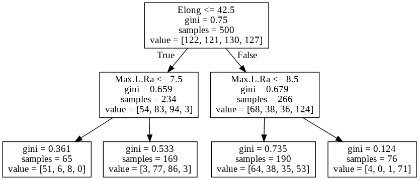
②モデルの可視化
dotデータを作成して、graphvizで樹形図が作成できます
import pydotplus
from IPython.display import Image
from graphviz import Digraph

dot_data = tree.export_graphviz(clf , feature_names = train_X.columns)
graph = pydotplus.graph_from_dot_data(dot_data)
Image(graph.create_png())
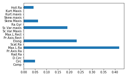
目的変数の重要度は、feature_importances_で出力
樹形図でもわかりますが、グラフの方が見やすい

print(clf.feature_importances_)

[0.         0.         0.         0.         0.         0.64321384
 0.         0.35678616 0.         0.         0.         0.
 0.         0.         0.         0.         0.         0.        ]

# グラフ作成
plt.barh(train_X.columns,clf.feature_importances_)
③改良/評価
1階層増やすだけなので結果のみにします
4分類で65%まで改善
トレーニングデータscore: 0.7
テストデータscore: 0.653179190751445
opelも分類できるようになりましたが、いまいちですね
混合行列
array([[88, 0, 6, 2],
[13, 17, 48, 13],
[11, 5, 54, 17],
[ 2, 0, 3, 67]])
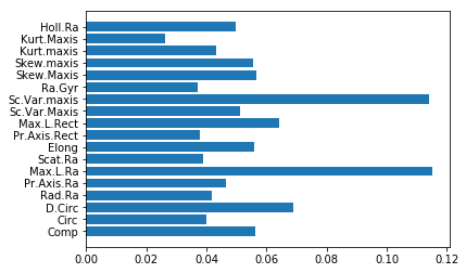
④可視化
説明変数もまんべんなく使うようになってます
⑤ランダムフォレストで実行/評価
scikit-learnは使い方が共通なのでimportした後は、ほぼ同じ使い方で便利です
テストデータスコアが0.72で伸びていますが、かなり過学習ですね
opelとsaabはランダムフォレストでも分類が難しい
説明変数そのままでは難しそうですね
次数ふやすか、SVMかはたまたDeeplearningか??等々と
すべての説明変数を使っています
# ランダムフォレスト
from sklearn.ensemble import RandomForestClassifier
clf_rf = RandomForestClassifier(random_state=0)
clf_rf = clf_rf.fit(train_X, train_y)
pred_rf = clf_rf.predict(test_X)

print('トレーニングデータscore:',clf_rf.score(train_X, train_y))
print('テストデータscore:',accuracy_score(pred_rf, test_y))

トレーニングデータscore: 0.99
テストデータscore: 0.7167630057803468

confusion_matrix(test_y, pred_rf)

array([[95,  0,  0,  1],
       [ 2, 49, 36,  4],
       [ 4, 35, 40,  8],
       [ 2,  1,  5, 64]])