ベイズ推論解析例題;:AとBのどちらが良いか
Pythonで体験するベイズ推論より
ベイズ推論でサイトAとサイトBのどちらが良いか?という問題です。
問題:サイトAの真のコンバージョンは?
サイトAを見たユーザーが最終的に資料請求や購入など利益につながるアクション(これをコンバージョンという)につながる確率を$p_A$とする。
$N$人がサイトAを見てそのうち$n$人がコンバージョンにつながったとする。
そうすると、
p_A=n/N
と思うかもしれないが、それは違う。つまり、$p_A$と$n/N$が等しいかどうかわからないからである。観測された頻度と真の頻度には差があり、真の頻度は事象が発生する確率と解釈できる。つまり、サイトAを見たから、アクションにつながったかどうかはわからないからである。
例えば、サイコロを例にとると、サイコロを振って1が出る真の頻度は$1/6$であるが、実際にサイコロを6回降っても一回も1が出ないかもしれない。それが観測された頻度である。
残念ながら現実は複雑すぎてノイズも避けられないので、真の頻度はわからないので、観測された頻度から真の頻度を推定するしかない。ベイズ統計から、事前分布と観測データ($n/N$)から真の頻度($p_A$)を推定するのである。
まず未知数$p_A$について事前分布を考えないといけない。データを持っていない時に、$p_A$をどう思っているか?まだ確信が持てないので、$p_A$は[0,1]の一様分布に従うと仮定しよう。
変数pに@pm.Uniformで、0から1の一様分布を与える.
import pymc3 as pm

# The parameters are the bounds of the Uniform.
with pm.Model() as model:
    p = pm.Uniform('p', lower=0, upper=1)
例えば、$p_A=0.05$であり、$N=1500$ユーザーがサイトAを見た時に、ユーザーがコンバージョン(サイトを見て購入や資料請求)したのが何人か、シミュレーションしてみよう。実際には$p_A$はわからないが、とりあえず知っていると仮定してシミュレーションして、観測データを作る。
N人がいるので、N回の試行のシミュレーションするために、ベルヌーイ分布を使う。ベルヌイー分布は二値変数(0か1かのどちらかを取る変数)についての確率分布であるため、コンバージョンしたか、しないかの計算に良い確率分布である。
X\sim \text{Ber}(p)
この時、$X$は確率$p$で$1$確率$1-p$で$0$である。
これをシミュレーションするpythonスクリプトは、
import scipy.stats as stats
import numpy as np

# set constants
p_true = 0.05  # remember, this is unknown.
N = 1500

# sample N Bernoulli random variables from Ber(0.05).
# each random variable has a 0.05 chance of being a 1.
# this is the data-generation step
occurrences = stats.bernoulli.rvs(p_true, size=N)

print(occurrences) # Remember: Python treats True == 1, and False == 0
print(np.sum(occurrences))

# [0 0 0 ... 0 0 0]
# 67

# Occurrences.mean is equal to n/N.
print("What is the observed frequency in Group A? %.4f" % np.mean(occurrences))
print("Does this equal the true frequency? %s" % (np.mean(occurrences) == p_true))

# What is the observed frequency in Group A? 0.0447
# Does this equal the true frequency? False
これで観測データ(occurrences)ができたので、観測データをPyMCのobs変数に設定して推論アルゴリズムを実行し、未知である$p_A$の事後分布のグラフを作る。
# include the observations, which are Bernoulli
with model:
    obs = pm.Bernoulli("obs", p, observed=occurrences)
    # To be explained in chapter 3
    step = pm.Metropolis()
    trace = pm.sample(18000, step=step,cores =1)
    burned_trace = trace[1000:]

import matplotlib.pyplot as plt
plt.title("Posterior distribution of $p_A$, the true effectiveness of site A")
plt.vlines(p_true, 0, 90, linestyle="--",color="r", label="true $p_A$ (unknown)")
plt.hist(burned_trace["p"], bins=25, histtype="bar",density=True)
plt.legend()
plt.show()
結果のグラフはこうなりました。
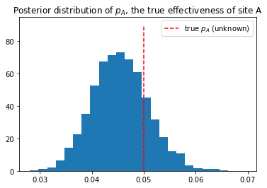
今回は、真の値の事前確率0.5に対し、事後確率のグラフはこのようなグラフになっています。これは繰り返せば、毎回微妙に違うグラフになります。
問題:サイトAとサイトBを比較すると、どちらが良いサイト?
サイトBも同様に計算すれば、$p_B$の事後確率を求めることができる。
またそこで、$delta=p_A-p_B$を計算することにした。
$p_A$と同様に$p_B$も真の値はわからない。仮に$p_B=0.4$とした。そうなると$delta=0.1$となる。先ほどの$p_A$と同様に$p_B$と$delta$を計算する。再度、すべてを計算してみた。
# -*- coding: utf-8 -*-

import pymc3 as pm
import scipy.stats as stats
import numpy as np
import matplotlib.pyplot as plt

# these two quantities are unknown to us.
true_p_A = 0.05
true_p_B = 0.04

# notice the unequal sample sizes -- no problem in Bayesian analysis.
N_A = 1500
N_B = 750

# generate some observations
observations_A = stats.bernoulli.rvs(true_p_A, size=N_A)
observations_B = stats.bernoulli.rvs(true_p_B, size=N_B)
print("Obs from Site A: ", observations_A[:30], "...")
print("Obs from Site B: ", observations_B[:30], "...")

# Obs from Site A:  [0 0 0 0 0 0 0 0 0 1 0 0 1 0 0 0 0 0 0 0 0 0 0 0 0 0 0 0 0 0] ...
# Obs from Site B:  [0 0 0 0 0 0 0 0 0 0 0 0 1 0 1 0 0 0 0 0 0 0 0 0 0 0 0 0 0 0] ...


print(np.mean(observations_A))
# 0.04666666666666667
print(np.mean(observations_B))
# 0.03866666666666667

# Set up the pymc3 model. Again assume Uniform priors for p_A and p_B.
with pm.Model() as model:
    p_A = pm.Uniform("p_A", 0, 1)
    p_B = pm.Uniform("p_B", 0, 1)

    # Define the deterministic delta function. This is our unknown of interest.
    delta = pm.Deterministic("delta", p_A - p_B)


    # Set of observations, in this case we have two observation datasets.
    obs_A = pm.Bernoulli("obs_A", p_A, observed=observations_A)
    obs_B = pm.Bernoulli("obs_B", p_B, observed=observations_B)

    # To be explained in chapter 3.
    step = pm.Metropolis()
    trace = pm.sample(20000, step=step,cores=1)
    burned_trace=trace[1000:]


p_A_samples = burned_trace["p_A"]
p_B_samples = burned_trace["p_B"]
delta_samples = burned_trace["delta"]

# histogram of posteriors

ax = plt.subplot(311)

plt.xlim(0, .1)
plt.hist(p_A_samples, histtype='stepfilled', bins=25, alpha=0.85,
         label="posterior of $p_A$", color="#A60628", density=True)
plt.vlines(true_p_A, 0, 80, linestyle="--", label="true $p_A$ (unknown)")
plt.legend(loc="upper right")
plt.title("Posterior distributions of $p_A$, $p_B$, and delta unknowns")

ax = plt.subplot(312)

plt.xlim(0, .1)
plt.hist(p_B_samples, histtype='stepfilled', bins=25, alpha=0.85,
         label="posterior of $p_B$", color="#467821", density=True)
plt.vlines(true_p_B, 0, 80, linestyle="--", label="true $p_B$ (unknown)")
plt.legend(loc="upper right")

ax = plt.subplot(313)
plt.hist(delta_samples, histtype='stepfilled', bins=30, alpha=0.85,
         label="posterior of delta", color="#7A68A6", density=True)
plt.vlines(true_p_A - true_p_B, 0, 60, linestyle="--",
           label="true delta (unknown)")
plt.vlines(0, 0, 60, color="black", alpha=0.2)
plt.legend(loc="upper right");

plt.show()

# Count the number of samples less than 0, i.e. the area under the curve
# before 0, represent the probability that site A is worse than site B.
print("Probability site A is WORSE than site B: %.3f" % \
    np.mean(delta_samples < 0))

print("Probability site A is BETTER than site B: %.3f" % \
    np.mean(delta_samples > 0))

# Probability site A is WORSE than site B: 0.201
# Probability site A is BETTER than site B: 0.799
結果のグラフはこうなった。
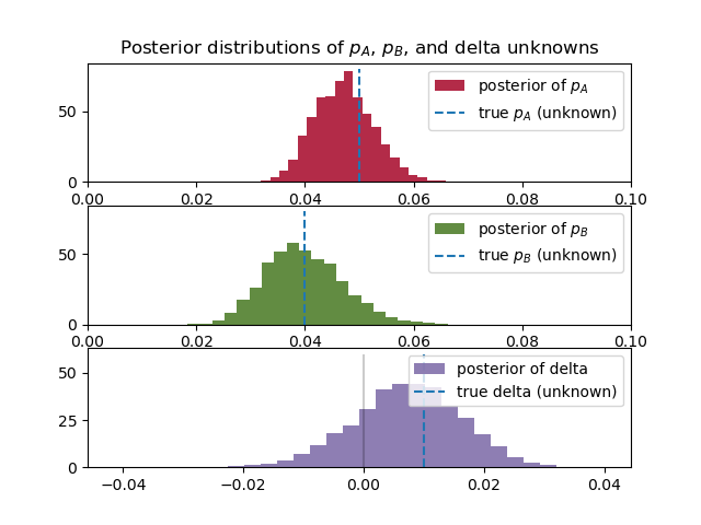
若干$p_B$の事後分布のすそ野が広いことがわかる。これはサイトBの方がデータが少ないためである。これは、サイトBのデータが少ないため、$p_B$の値に自信が持てないことを示している。
また、3つ目のグラフ$delta=p_A-p_B$は、0より大きい値を示している。これはつまりサイトAの方がコンバージョンとしてユーザーの反応が良いことを示している。
$p_A$、$p_B$やデータ数の値を変えて計算をすると、より理解が深まります。