「実践コンピュータビジョン」の全演習問題をやってみた。詳細編 第３章 画像間の写像

まえおき

先日投稿した「実践コンピュータビジョン」の全演習問題をやってみたの詳細です。なお、あくまで「やってみた」であって、模範解答ではありません。「やってみた」だけなので、うまくいかなかった、という結果もあります。

この記事は「実践コンピュータビジョン」（オライリージャパン、Jan Erik Solem著、相川愛三訳）の演習問題に関する記事です。この記事を書いた人間と書籍との間には何の関係もありません。著者のJan氏と訳者の相川氏にはコンピュータビジョンについて学ぶ機会を与えて頂いたことに感謝します。

実践コンピュータビジョンの原書("Programming Computer Vision with Python")の校正前の原稿は著者のJan Erik Solem氏がCreative Commons Licenseの元で公開されています。。

回答中で使用する画像の多く、また、sfm.py, sift.py, stereo.pyなどの教科書中で作られるファイルはこれらのページからダウンロードできます。
オライリージャパンのサポートページ
Jan Erik Solem氏のホームページ
相川愛三氏のホームページ

ここで扱うプログラムはすべてPython2.7上で動作を確認しています。一部の例外を除きほとんどがJupyter上で開発されました。また必要なライブラリーを適宜インストールしておく必要があります。Jupyter以外の点は、上記の書籍で説明されています。

結構な分量なので章毎に記事をアップしています。今回は第３章です。

３章　画像感の写像

アフィン変換やホモグラフィー、RANSAC、パノラマの作成などがあります。楽しみです。
なお、imregistration.py中rigid_alignmentという関数の精度が出ず修正しました。

元はこのようなコードです。

  for i in range(len(im.shape)):
    im2[:,:,i] = ndimage.affine_transform(im[:,:,i],linalg.inv(T),offset=[-ty,-tx])

いろいろ試したのですが、変形の際にスケールも考慮に入れたほうが良いようです。

  s = math.sqrt(R[0][0]**2+R[0][1]**2) # this is not in the text book but needed
  for i in range(len(im.shape)):
    im2[:,:,i] = ndimage.affine_transform(im[:,:,i],linalg.inv(T),offset=[-ty/s,-tx/s])

では問題に入ります。

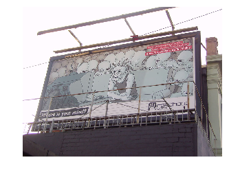
3.4.1 Create a function that takes the image coordinates of a square (or rectangular) object, for example a book, a poster or a 2D bar code, and estimates the transform that takes the rectangle to a full on frontal view in a normalized coordinate system. Use ginput() or the strongest Harris corners to find the points.

斜めから見た正方形や長方形の画像を見つけて、正面から見た形になおしましょう。

私の回答

教科書内で作ったライブラリのwarp.pyとhomography.pyを使います。
https://github.com/moizumi99/CVBookExercise/blob/master/Chapter-3/CV%20Book%20CH%203%20Ex%201.ipynb

from PIL import Image
from numpy import *
from pylab import *
from scipy import ndimage
import warp
import homography

im1 = array(Image.open('billboard1.jpg'))
imshow(im1)
gray()
axis('off')
show()

im2 = zeros((400, 700, 3))
m, n, cn = im2.shape

fp = array([[223, 494, 441, 126], [128, 60, 719, 717], [1, 1, 1, 1]])
tp = array([[0, m, m, 0], [0, 0, n, n], [1, 1, 1, 1]])

tp2 = tp[:, :3]
fp2 = fp[:, :3]
H = homography.Haffine_from_points(tp2, fp2)

im3 = zeros((400, 700, 3))
for color in range(3):
    im1_t = ndimage.affine_transform(im1[:, :, color], H[:2, :2], (H[0,2],H[1,2]), im2.shape[:2])
    alpha = warp.alpha_for_triangle(tp2, im2.shape[0], im2.shape[1])
    im3[:, :, color] = (1-alpha)*im2[:, :, color] + alpha*im1_t

tp2 = tp[:, [0,2,3]]
fp2 = fp[:, [0,2,3]]
H = homography.Haffine_from_points(tp2, fp2)

im4 = zeros((400, 700, 3))
for color in range(3):
    im1_t = ndimage.affine_transform(im1[:, :, color], H[:2, :2], (H[0,2],H[1,2]), im2.shape[:2])

    alpha = warp.alpha_for_triangle(tp2, im2.shape[0], im2.shape[1])
    im4[:, :, color] = (1-alpha)*im3[:, :, color] + alpha*im1_t

figure(figsize=(12, 8))
#gray()
imshow(uint8(im4))
axis('equal')
axis('off')
show()

ほぼ教科書そのままです。もとが平面なら結構綺麗にもどるものです。
なお画像位置([223, 494, 441, 126], [128, 60, 719, 717])は画像編集ソフトを使って手作業で探しました。

3.4.2 Write a function that correctly determines the alpha map for a warp like the one in Figure 3.1.

これは多分"the one in Figure 3.2"の間違いなのではないかなと思っています。Figure 3.2は別の画像をはめ込む処理です。

私の回答

from PIL import Image
from numpy import *
from pylab import *
from scipy import ndimage
import warp
import homography


im1 = array(Image.open('cat.jpg').convert('L'))
im1[100:200, 300:400] = 0
im2 = array(Image.open('bill_board_for_rent.jpg').convert('L'))
tp = array([[264, 538, 540, 264],[40, 36, 605, 605],[1, 1,1,1]])
#tp = array([[675, 826, 826, 677],[55, 52, 281, 277],[1, 1,1,1]])
im3 = warp.image_in_image(im1, im2, tp)
figure(figsize=(12, 12))
gray()
imshow(im3)
axis('equal')
axis('off')
show()

画像に穴を開けるためにわざわざim1[100:200, 300:400] = 0のようなことをしています。この部分は透明で後ろの風景がすけるはずです。黒い筋が残ってしまいました。まだ改善の余地があります。
何にせよ、問題の意図がいまだにちょっとわからず、これでそもそも正しい方向に向かっているのかさえわかりません。

3.4.3 Find a data set of your own that contains three common landmark points (like in the face example or using a famous object like the Eiffel tower). Create aligned images where the landmarks are in the same position. Compute mean and median images and visualize them.

３つの基準点を含むデータセットを使って、位置合わせをしてmean画像とmedian画像をつくります。

私の回答

この演習のためにfacial-landmarks.zipという顔画像とランドマークのセットになったデータをダウンロードしてきて使ったのですが、どこからダウンロードしたのか失念してしまいました。

from PIL import Image
from numpy import *
from pylab import *
import imregistration
import imtools
import os
from scipy import ndimage
from scipy.misc import imsave
import os

def read_points_from_pts(dir):
    files = imtools.get_imlist(dir)
    faces = {}
    for path in files:
        fileName = os.path.basename(path)
        base = os.path.splitext(path)[0]
        txtfile = base + ".pts"
        f = open(txtfile, 'r')
        for i in range(3+68):
            line = f.readline()
            if (i==3+37):
                p1 = line.split()
            elif (i==3+46):
                p2 = line.split()
            elif (i==3+58):
                p3 = line.split()
        xf = int(float(p1[0]))
        yf = int(float(p1[1]))
        xs = int(float(p2[0]))
        ys = int(float(p2[1]))
        xm = int(float(p3[0]))
        ym = int(float(p3[1]))
        faces[fileName]=array([xf, yf, xs, ys, xm, ym])
    return faces
def rigid_alignment1(faces,path,plotflag=False):
    """ Align images rigidly and save as new images.
    path determines where the aligned images are saved.
    set plotflag=True to plot the images. """

    refpoints = faces.values()[0]
    wm = 2000
    hm = 2000

    import math

    for face in faces:
        points = faces[face]

        #print "refpoints: ", refpoints, "\n"
        #print "points:    ", points, "\n"

        R,tx,ty = imregistration.compute_rigid_transform(refpoints,points)
        #print "R: ", R, "\n"
        #print "(tx, ty): ", (tx, ty), "\n"

        ## Scale is not in the text book but needed
        s = math.sqrt(R[0][0]**2+R[0][1]**2)
        #print "Scale: ", s, "\n"

        T = array([[R[1][1], R[1][0]], [R[0][1], R[0][0]]])

        im = array(Image.open(os.path.join(path,face)))
        im1 = zeros([wm, hm, 3])
        m, n, c = im.shape
        m = min(wm, m)
        n = min(hm, n)
        c = min(3, c)
        im1[0:m, 0:n, 0:c] = im[0:m, 0:n, 0:c]
        im2 = zeros(im1.shape, 'uint8')

        # Per color channel
        for i in range(len(im.shape)):
            im2[:, :, i] = 
ndimage.affine_transform(im1[:,:,i],linalg.inv(T),
                                                    offset=[-ty/s,-tx/s])
            # need to normalize the trainsition with scale
        if plotflag:
            imshow(im2)
            show()

        im2 = uint8(im2)
        h,w = im2.shape[:2]
        outsize = 1024
        border = 128
        imsave(os.path.join(path, 'aligned/'+face),
               im2[border:outsize+border,border:outsize+border,:])

points = read_points_from_pts('../faces/trainset/')
rigid_alignment1(points, '../faces/trainset/')

from pylab import *
import imtools

dir = '../faces/trainset/aligned/'
imlist = imtools.get_imlist(dir)
avgimg = imtools.compute_average(sorted(imlist))
figure()
imshow(avgimg)
gray()
axis('off')
title(dir)

show()

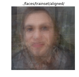
こ、これはどうなんでしょうか。老若男女問わず含んだデータベースなのでこんなものかもしれませんが...。もっと適切なデータがないと改善は難しいかもしれません。この画像をみてやる気をなくして、メディアンイメージはやっていません。
なお、教科書内のrigid_alignment関数の代わりにスケーリングを修正したrigid_alignment1関数を作って使用しています。こうしておかないともっと酷いことになります。

3.4.4 Implement intensity normalization and a better way to blend the images in the panorama example to remove the edge effects in Figure 3.12.

輝度の正規化を行い、Figure 3.12のエッジ効果を改善しなさい

私の回答

from PIL import Image
from numpy import *
from pylab import *
import ransac
import sift
from PIL import Image
import homography
import warp

featname = ['Univ'+str(i+1)+'.sift' for i in range(5)]
imname = ['Univ'+str(i+1)+'.jpg' for i in range(5)]
l = {}
d = {}
for i in range(5):
    sift.process_image(imname[i],featname[i])
    l[i],d[i] = sift.read_features_from_file(featname[i])
    l[i][:,[0,1]] = l[i][:,[1,0]]

matches = {}
for i in range(4):
    matches[i] = sift.match(d[i+1],d[i])

def convert_points(j):
    ndx = matches[j].nonzero()[0]
    fp = homography.make_homog(l[j+1][ndx, :2].T)
    ndx2 = [int(matches[j][i]) for i in ndx]
    tp = homography.make_homog(l[j][ndx2,:2].T)
    return fp, tp

model = homography.RansacModel()

fp, tp = convert_points(1)
H_12 = homography.H_from_ransac(fp, tp, model)[0] #im1 to im2

fp, tp = convert_points(0)
H_01 = homography.H_from_ransac(fp, tp, model)[0] #im0 to im1

tp, fp = convert_points(2)
H_32 = homography.H_from_ransac(fp, tp, model)[0] #im3 to im2

tp, fp = convert_points(3)
H_43 = homography.H_from_ransac(fp, tp, model)[0] #im4 to im3

# no brightness adjustment

delta = 2000


im1 = array(Image.open(imname[1]))
im2 = array(Image.open(imname[2]))
im_12 = warp.panorama(H_12, im1, im2, delta, delta)

im1 = array(Image.open(imname[0]))
im_02 = warp.panorama(dot(H_12, H_01), im1, im_12, delta, delta)

im1 = array(Image.open(imname[3]))
im_32 = warp.panorama(H_32, im1, im_02, delta, delta)

im1 = array(Image.open(imname[4]))
im_42 = warp.panorama(dot(H_32, H_43), im1, im_32, delta, 2*delta)
im_42[im_42<0] = 0
im_42[im_42>255] = 255
im_42 = uint8(im_42)

figure(figsize=(12,12))
imshow(uint8(im_42))
axis('off')
show()

#brightness adjustment

delta = 2000

im0 = array(Image.open(imname[0]))
im1 = array(Image.open(imname[1]))
im2 = array(Image.open(imname[2]))
im3 = array(Image.open(imname[3]))
im4 = array(Image.open(imname[4]))

im2 = im2 * 128.0/(im2.mean())
im1 = im1 * (im2[:, im2.shape[1]/2:]).mean()/(im1[:, :im1.shape[1]/2]).mean()
im0 = im0 * (im1[:, im1.shape[1]/2:]).mean()/(im0[:, :im0.shape[1]/2]).mean()
im3 = im3 * (im2[:, :im2.shape[1]/2]).mean()/(im3[:, im3.shape[1]/2:]).mean()
im4 = im4 * (im3[:, :im3.shape[1]/2]).mean()/(im4[:, im4.shape[1]/2:]).mean()


im_12 = warp.panorama(H_12, im1, im2, delta, delta)
im_02 = warp.panorama(dot(H_12, H_01), im0, im_12, delta, delta)
im_32 = warp.panorama(H_32, im3, im_02, delta, delta)
im_42 = warp.panorama(dot(H_32, H_43), im4, im_32, delta, 2*delta)
im_42[im_42<0] = 0
im_42[im_42>255] = 255
im_42 = uint8(im_42)

figure(figsize=(12,12))
imshow(uint8(im_42))
axis('off')
show()

上が輝度調整前、下が輝度調整後、なのですがあまり変わってないですね。
右端の黒い部分は左右の処理を対称にするために入れたブランク部分です。

3.4.5 Instead of warping to a central image, panoramas can be created by warping on to a cylinder. Try this for the example in Figure 3.12.

Figure 3.12の例を使って、円筒状にパノラマを作りなさい。

私の回答

円筒状というのは、平面に３６０度の視野をマップするかわりに、円筒の表面にマップするという意味だと解釈しました。結局は左右の端がつながったパノラマ、ということになるかと思います。そうなると、Figure 3.12の画像は数が足りず、３６０度分ありません。
そこで、コーネル大学のデータベースを借りることにしました。
http://www.cs.cornell.edu/courses/cs6670/2011sp/projects/p2/project2.html
こちらから、pano_test.zipをダウンロードして使用しています。

from PIL import Image
from numpy import *
from pylab import *
import ransac
import sift
from PIL import Image
import homography
import warp
from scipy import ndimage

def Hsimilarity_from_points(fp, tp):
    """ Find similarity transformation, such that fp is mapped to tp
    using the linear DLT method. Points are conditioned
    automatically. """

    if fp.shape != tp.shape:
        raise RuntimeError('number of points do not match')

    # Condition points (important for numerical reasons)
    # --from points--
    m = mean(fp[:2], axis=1)
    maxstd = max(std(fp[:2], axis=1)) + 1e-9
    C1 = diag([1/maxstd, 1/maxstd, 1])
    C1[0][2] = -m[0]/maxstd
    C1[1][2] = -m[1]/maxstd
    fp = dot(C1, fp)

    # -- to points --
    m = mean(tp[:2], axis=1)
    maxstd = max(std(tp[:2], axis=1)) + 1e-9
    C2 = diag([1/maxstd, 1/maxstd, 1])
    C2[0][2] = -m[0]/maxstd
    C2[1][2] = -m[1]/maxstd
    tp = dot(C2, tp)

    # create matrix for linear method
    # Start from similarity transformation,
    # [x', y', 1].T = [[c, -s, tx], [s, c, ty], [0, 0, 1]] * [x, y, 1]
    # c = a*cos(t)
    # s = a*sin(t)
    # this can be extended to 
    # [[(x*y'-y*x'), -(x*x'+y*y'), y', -x']*[c, s, tx, ty]=[0, 0, 0].T
    # (.T is transverse)
    # By solving this for [(x, y, x', y') = [[x1, y1, x1', y1'], [x2, y2, x2', y2'], ...]
    # You can get c, s, tx, ty : similarity matrix
    nbr_correspondences = fp.shape[1]
    A = zeros((nbr_correspondences, 4))
    for i in range(nbr_correspondences):
        A[i] = [fp[0][i]*tp[1][i]-fp[1][i]*tp[0][i], -fp[0][i]*tp[0][i]-fp[1][i]*tp[1][i], tp[1][i], -tp[0][i]]
        U, S, V = linalg.svd(A)
        H = [[V[3][0], -V[3][1], V[3][2]], [V[3][1], V[3][0], V[3][3]], [0, 0, 1]]
        # V[3] has the smallest singlarity value = smallest error in least square method
    # decondition (C1, C2)
    H = dot(linalg.inv(C2), dot(H, C1))

    # normalize and return
    return H

class RansacModel_2(object):
    """ Class for testing homography fit with ransac.py from
    http://www.scipy.org/Cookbook/RANSAC
    This version uses Similarity Transformation 
    """

    def __init__(self, debug=False):
        self.debug = debug

    def fit(self, data):
        """ Fit homography to four selected correspondences. """

        data = data.T

        fp = data[:3, :4]

        tp = data[3:, :4]

        return Hsimilarity_from_points(fp,tp)

    def get_error(self, data, H):
        """ Apply homography to all correspondences,
        return error for each transformed point."""

        data = data.T

        fp = data[:3]
        tp = data[3:]


        fp_transformed = dot(H, fp)

        #
        nz = nonzero(fp_transformed[2])
        for i in range(3):
            fp_transformed[i][nz] /= fp_transformed[2][nz]

        return sqrt(sum((tp-fp_transformed)**2, axis=0))

# use the test data here
# http://www.cs.cornell.edu/courses/cs6670/2011sp/projects/p2/project2.html

featname = ['campus_0'+('0' if (i<10) else '')+str(i)+'.sift' for i in range(18)]
imname = ['campus_0'+('0' if (i<10) else '')+str(i)+'.jpg' for i in range(18)]
l = {}
d = {}
for i in range(18):
    sift.process_image(imname[i],featname[i])
    l[i],d[i] = sift.read_features_from_file(featname[i])
    l[i][:,[0,1]] = l[i][:,[1,0]]

matches = {}
for i in range(18):
    matches[i] = sift.match(d[(i+1)%18],d[i])

def convert_points(j):
    ndx = matches[j].nonzero()[0]
    fp = homography.make_homog(l[(j+1)%18][ndx, :2].T)
    ndx2 = [int(matches[j][i]) for i in ndx]
    tp = homography.make_homog(l[j][ndx2,:2].T)
    return fp, tp

model = RansacModel_2()

#H = [[[0,0,0],[0,0,0],[0,0,0]] for i in range(18)]
H = []
for i in range(18):
    fp, tp = convert_points(i)
    H.append(homography.H_from_ransac(fp, tp, model)[0]) #im1 to im2

delta = 480
st = 18
vdelta = 120
im1 = array(Image.open(imname[st%18]))
im1 = 128.0*im1/np.average(im1)
im1 = vstack((im1, zeros((vdelta, im1.shape[1], im1.shape[2]))))
#im1 = vstack((zeros((vdelta, im1.shape[1], im1.shape[2])), im1))

def transf(p):
    p2 = dot(H, [p[0], p[1], 1])
    return (p2[0]/p2[2], p2[1]/p2[2])

ty = 0
tx = 0
H1 = array([[1, 0, 0], [0, 1, 0], [0, 0, 1]])
delta = 640
for i in range(st, 0, -1):
    i = i % 18
    j = i-1 if (i>0) else 18+i-1
    print "From "+str(i)+" to "+str(j)+"\n"
    im2 = array(Image.open(imname[j]))
    [m, n, c] = im2.shape
    im2 = 128.0*im2/np.average(im2)
    im2 = vstack((im2, zeros((vdelta, n, im2.shape[2]))-100))
    H1 = dot(H[j], H1)
    delta = uint16(640 - (im1.shape[1] + H1[1][2] - 480))
    delta = 0 if (delta<0) else delta
    im0 = zeros(im1.shape)-100
    im2 = warp.panorama(H1, im2, im0, delta, delta)
    im1 = hstack((im1, zeros((im1.shape[0], delta, 3))))

    # Adjust the perspective 
    # [m, n, c] = im2.shape
    op = array([[0, 0, m, m], [0, n, n, 0], [1, 1, 1, 1]])
    fp = dot(inv(H1), op)
    tx = math.sqrt((fp[0][1]-fp[0][0])**2 + (fp[1][1]-fp[1][0])**2)
    tp = array([[fp[0][0], op[0][1], op[0][2], fp[0][3]], [fp[1][0], fp[1][0]+tx, fp[1][0]+tx, fp[1][3]], [1, 1, 1, 1]])

    tp2 = tp[:, [0, 2, 3]]
    fp2 = fp[:, [0, 2, 3]]
    H2 = homography.Haffine_from_points(tp2, fp2)
    im3 = zeros(im1.shape)
    for c in range(3):
        im3[:,:,c] = ndimage.affine_transform(im2[:,:,c], H2[:2,:2], (H2[0,2], H2[1,2]), im1.shape[:2])

    tp2 = tp[:, [0, 1, 2]]
    fp2 = fp[:, [0, 1, 2]]
    H2 = homography.Haffine_from_points(tp2, fp2)
    im4 = zeros(im1.shape)
    for c in range(3):
        im4[:,:,c] = ndimage.affine_transform(im2[:,:,c], H2[:2,:2], (H2[0,2], H2[1,2]), im1.shape[:2])

    im1[im3>=0] = im3[im3>=0]
    im1[im4>=0] = im4[im4>=0]

    H1 = dot(H1, H2)
    imshow(uint8(im1))
    axis('off')
    show()    

im1[im1<0] = 0
im1[im1>255] = 255
im1 = uint8(im1)

figure(figsize=(12,12))
imshow(uint8(im1))
axis('off')
show()

figure(figsize=(16,16))
imshow(uint8(im1))
axis('off')
show()

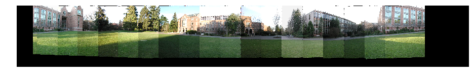
最初に作った時は、画像を左右に足していくにつれて上に上がってしまい、だんだん円のような形になってしまいました。おそらくもとの画像の撮影条件のせいではないかと考えています。このバージョンでは、新しい画像を足すたびにアフィン変換して、全体の方向を水平に戻しています。

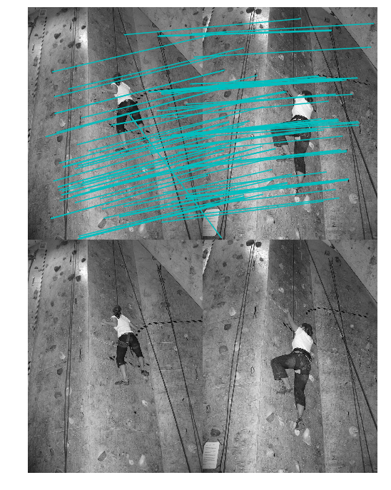
3.4.6 Use RANSAC to find several dominant homography inlier sets. An easy way to do this is to first make one run of RANSAC, find the homograohy with the largest consistent subset, then remove the inliers from the set of matches, then run RANSAC again to get the next biggest set, and so on.

RANSACを使って、ドミナントなホモグラフィーインライアーを複数見つけなさい。

私の回答

問題分のサジェスチョンにしたがって、RANSACを使って最適なインライアを見つけ、集合から除去し、またRANSACを使う、という処理を繰り返しています。

from PIL import Image
from numpy import *
from pylab import *
import ransac
import sift
import harris
import homography

featname = ['climbing_'+str(i+1)+'_small.sift' for i in range(2)]
imname = ['climbing_'+str(i+1)+'_small.jpg' for i in range(2)]
l = {}
d = {}
for i in range(2):
    sift.process_image(imname[i],featname[i])
    l[i],d[i] = sift.read_features_from_file(featname[i])
#    l[i][:,[0,1]] = l[i][:,[1,0]]

matches = {}
for i in range(1):
    matches[i] = sift.match(d[i+1],d[i])

def convert_points(j):
    ndx = matches[j].nonzero()[0]
    fp = homography.make_homog(l[j+1][ndx, :2].T)
    ndx2 = [int(matches[j][i]) for i in ndx]
    tp = homography.make_homog(l[j][ndx2,:2].T)
    return fp, tp


im = [array(Image.open(imname[i]).convert('L')) for i in range(2)]
for i in range(1):
    figure(figsize=(12,12))
    gray()
    sift.plot_matches(im[i+1],im[i],l[i+1],l[i],matches[i])
show()

m = homography.RansacModel()
fp, tp = convert_points(0)
tp1 = []
for i in range(3):
    H, rd = homography.H_from_ransac(fp, tp, m, 1000,5)
    fp1.append(fp[:, rd])
    tp1.append(tp[:, rd])
    fp = np.delete(fp, rd, axis=1)
    tp = np.delete(tp, rd, axis=1)

im = [array(Image.open(imname[i]).convert('L')) for i in range(2)]
figure(figsize=(12,12))
gray()
im3 = harris.appendimages(im[0], im[1])
imshow(im3)

for t in range(len(fp1)):
    cols = im[0].shape[1]
    colors = ['c', 'g', 'r', 'k']
    for i in range(len(fp1[t][0])):
        plot([fp1[t][0][i], tp1[t][0][i]+cols], [fp1[t][1][i], tp1[t][1][i]], colors[t])
axis('off')
show()

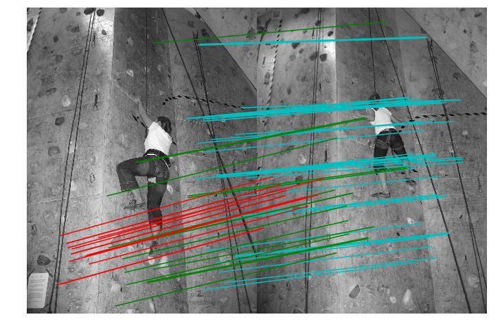
ドミナントなホモグラフィーごとに色分けしてあります

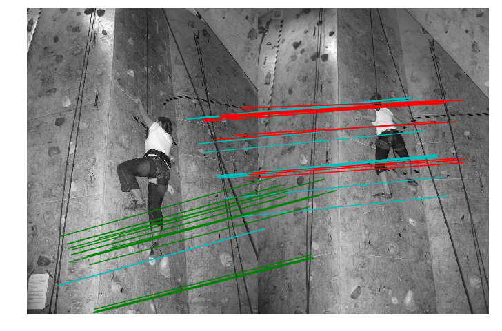
3.4.7 Modify the homography RANSAC estimation to instead estimate affine transformations using three point correspondences. Use this to determine if a pair of images contains a planar scene, for example using the inlier count. A planar scene will have a high inlier count for an affine transformation.

RANSACを使い、ホモグラフィーの代わりにアフィン変換を推定します。２枚の画像が１つの平面を共有するか判別しなさい。

私の回答

from PIL import Image
from numpy import *
from pylab import *
import ransac
import sift
import harris
import homography

featname = ['climbing_'+str(i+1)+'_small.sift' for i in range(2)]
imname = ['climbing_'+str(i+1)+'_small.jpg' for i in range(2)]
l = {}
d = {}
for i in range(2):
    sift.process_image(imname[i],featname[i])
    l[i],d[i] = sift.read_features_from_file(featname[i])
#    l[i][:,[0,1]] = l[i][:,[1,0]]

matches = {}
for i in range(1):
    matches[i] = sift.match(d[i+1],d[i])

def convert_points(j):
    ndx = matches[j].nonzero()[0]
    fp = homography.make_homog(l[j+1][ndx, :2].T)
    ndx2 = [int(matches[j][i]) for i in ndx]
    tp = homography.make_homog(l[j][ndx2,:2].T)
    return fp, tp

im = [array(Image.open(imname[i]).convert('L')) for i in range(2)]
for i in range(1):
    figure(figsize=(12,12))
    gray()
    sift.plot_matches(im[i+1],im[i],l[i+1],l[i],matches[i])
show()

class RansacModel2(object):
    """ Class for testing homography fit with ransac.py from
    http://www.scipy.org/Cookbook/RANSAC"""

    def __init__(self, debug=False):
        self.debug = debug

    def fit(self, data):
        """ Fit homography to four selected correspondences. """

        data = data.T

        fp = data[:3, :4]

        tp = data[3:, :4]

        return homography.Haffine_from_points(fp, tp)

    def get_error(self, data, H):
        """ Apply homography to all correspondences,
        return error for each transformed point."""

        data = data.T

        fp = data[:3]
        tp = data[3:]


        fp_transformed = dot(H, fp)

        #
        nz = nonzero(fp_transformed[2])
        for i in range(3):
            fp_transformed[i][nz] /= fp_transformed[2][nz]

        return sqrt(sum((tp-fp_transformed)**2, axis=0))

m = RansacModel2()
fp, tp = convert_points(0)
fp1 = []
tp1 = []
for i in range(3):
    H, rd = homography.H_from_ransac(fp, tp, m, 1000, 5)
    fp1.append(fp[:, rd])
    tp1.append(tp[:, rd])
    fp = np.delete(fp, rd, axis=1)
    tp = np.delete(tp, rd, axis=1)

im = [array(Image.open(imname[i]).convert('L')) for i in range(2)]
figure(figsize=(12,12))
gray()
im3 = harris.appendimages(im[0], im[1])
imshow(im3)
for t in range(len(fp1)):
    cols = im[0].shape[1]
    colors = ['c', 'g', 'r', 'k']
    for i in range(len(fp1[t][0])):
        plot([fp1[t][0][i], tp1[t][0][i]+cols], [fp1[t][1][i], tp1[t][1][i]], colors[t])
axis('off')
show()

print len(fp1[0][0])
print len(fp1[1][0])
print len(fp1[2][0])

18
15
19

同一平面を共有する点の組ごとに色分けしてあります。同一平面上の点の数は、18, 15, 19でした。（乱数を使っているので、試行毎に変わります）
これは多いと言えるのでしょうか？たぶん十分だとは思いますが、わかりません。

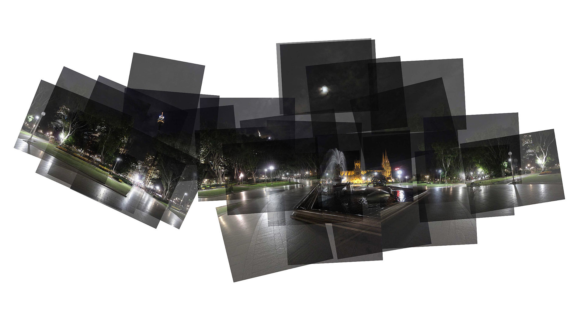
3.8 Build a panograph (http://en.wikipedia.org/wiki/Panography) from a collection (for example from Flickr) by matching local features and using leastsquares rigid registration.

パノグラフをつくりなさい。

パノグラフというのは、複数の画像を組み合わせて作った大きなサイズの画像です。２次元パノラマといってもいいかもしれません。例としてはこのようなものがあります（クリエイティブコモンズライセンス下で公開されている例です）

私の回答

from PIL import Image
from numpy import *
from pylab import *
import ransac
import sift
from PIL import Image
import homography
import warp
from scipy import ndimage
import os
import scipy.misc

def Hsimilarity_from_points(fp, tp):
    """ Find similarity transformation, such that fp is mapped to tp
    using the linear DLT method. Points are conditioned
    automatically. """

    if fp.shape != tp.shape:
        raise RuntimeError('number of points do not match')

    # Condition points (important for numerical reasons)
    # --from points--
    m = mean(fp[:2], axis=1)
    maxstd = max(std(fp[:2], axis=1)) + 1e-9
    C1 = diag([1/maxstd, 1/maxstd, 1])
    C1[0][2] = -m[0]/maxstd
    C1[1][2] = -m[1]/maxstd
    fp = dot(C1, fp)

    # -- to points --
    m = mean(tp[:2], axis=1)
    maxstd = max(std(tp[:2], axis=1)) + 1e-9
    C2 = diag([1/maxstd, 1/maxstd, 1])
    C2[0][2] = -m[0]/maxstd
    C2[1][2] = -m[1]/maxstd
    tp = dot(C2, tp)

    # create matrix for linear method
    # Start from similarity transformation,
    # [x', y', 1].T = [[c, -s, tx], [s, c, ty], [0, 0, 1]] * [x, y, 1]
    # c = a*cos(t)
    # s = a*sin(t)
    # this can be extended to 
    # [[(x*y'-y*x'), -(x*x'+y*y'), y', -x']*[c, s, tx, ty]=[0, 0, 0].T
    # (.T is transverse)
    # By solving this for [(x, y, x', y') = [[x1, y1, x1', y1'], [x2, y2, x2', y2'], ...]
    # You can get c, s, tx, ty : similarity matrix
    nbr_correspondences = fp.shape[1]
    A = zeros((nbr_correspondences, 4))
    for i in range(nbr_correspondences):
        A[i] = [fp[0][i]*tp[1][i]-fp[1][i]*tp[0][i], -fp[0][i]*tp[0][i]-fp[1][i]*tp[1][i], tp[1][i], -tp[0][i]]
#        A[i] = [fp[1][i]*tp[0][i]-fp[0][i]*tp[1][i], -fp[1][i]*tp[1][i]-fp[0][i]*tp[0][i], tp[0][i], -tp[1][i]]
    U, S, V = linalg.svd(A)
    H = [[V[3][0], -V[3][1], V[3][2]], [V[3][1], V[3][0], V[3][3]], [0, 0, 1]]
        # V[3] has the smallest singlarity value = smallest error in least square method
    # decondition (C1, C2)
    H = dot(linalg.inv(C2), dot(H, C1))

    # normalize and return
    return H

class RansacModel_2(object):
    """ Class for testing homography fit with ransac.py from
    http://www.scipy.org/Cookbook/RANSAC
    This version uses Similarity Transformation 
    """

    def __init__(self, debug=False):
        self.debug = debug

    def fit(self, data):
        """ Fit homography to four selected correspondences. """

        data = data.T

        fp = data[:3, :4]

        tp = data[3:, :4]

#       return Hsimilarity_from_points(fp,tp)
        return homography.Haffine_from_points(fp,tp)

    def get_error(self, data, H):
        """ Apply homography to all correspondences,
        return error for each transformed point."""

        data = data.T

        fp = data[:3]
        tp = data[3:]


        fp_transformed = dot(H, fp)

        #
        nz = nonzero(fp_transformed[2])
        for i in range(3):
            fp_transformed[i][nz] /= fp_transformed[2][nz]

        return sqrt(sum((tp-fp_transformed)**2, axis=0))

# use the test data here
# http://www.cs.cornell.edu/courses/cs6670/2011sp/projects/p2/project2.html
# Yosemite set
# other files are here, but not used now
# http://www.cvl.isy.liu.se/en/research/datasets/passta/
def extract_matches(img1, img2):
    img_name = [os.path.splitext(img1)[0], os.path.splitext(img2)[0]]
    ext_name = [os.path.splitext(img1)[1], os.path.splitext(img2)[1]]
    featname = [img_name[i]+'.sift' for i in range(2)]
    iname = [img_name[i]+ext_name[i] for i in range(2)]
    l = {}
    d = {}
    for i in range(2):
        sift.process_image(iname[i],featname[i])
        l[i],d[i] = sift.read_features_from_file(featname[i])
        l[i][:,[0,1]] = l[i][:,[1,0]]

    matches = sift.match(d[1],d[0])
    return l, d, matches

def convert_points(matches, l):
    ndx = matches.nonzero()[0]
    fp = homography.make_homog(l[1][ndx, :2].T)
    ndx2 = [int(matches[i]) for i in ndx]
    tp = homography.make_homog(l[0][ndx2,:2].T)
    return fp, tp

debug=False

imname = ['./yosemite_test/yosemite1.jpg', 
          './yosemite_test/yosemite2.jpg', 
          './yosemite_test/yosemite3.jpg', 
          './yosemite_test/yosemite4.jpg']

tmpname = 'tmpimg0.png'

first_img = True
for imn1 in range(0, 3):
    imname1 = imname[imn1] if (first_img) else tmpname
    im1 = array(Image.open(imname1)) # if (first_img) else im1_t
    first_img = False
    imn2 = imn1+1
    im2 = array(Image.open(imname[imn2]))
    l, d, matches = extract_matches(imname[imn2], imname1)
    fp, tp = convert_points(matches, l)

    model = RansacModel_2()
    # model = homography.RansacModel()
    H, inlier = homography.H_from_ransac(fp, tp, model)
    # print H

    m, n, c = im2.shape
    op = [[0, 0, m, m], [0, n, n, 0], [1, 1, 1, 1]]
    dp = dot(inv(H), op)

    ymax = int(max(dp[0]))
    ymin = int(min(dp[0]))
    xmax = int(max(dp[1]))
    xmin = int(min(dp[1]))

    xleft = 0 if (xmin>0) else -xmin
    xright = 0 if (xmax<im1.shape[1]) else (xmax-im1.shape[1])
    ytop = 0 if (ymin>0) else -ymin
    ybot = 0 if (ymax<im1.shape[0]) else (ymax-im1.shape[0])

    ty = -ytop
    tx = -xleft
    im1 = hstack((zeros((im1.shape[0], xleft, c)), im1, zeros((im1.shape[0], xright, c))))
    im1 = vstack((zeros((ytop, im1.shape[1], c)), im1, zeros((ybot, im1.shape[1], c))))

    if (debug==True):
        print "op\n", op
        print "dp\n", dp
        print 'ymax', ymax
        print 'ymin', ymin
        print 'xmax', xmax
        print 'xmin', xmin
        print 'ytop', ytop
        print 'ybot', ybot
        print 'xleft', xleft
        print 'xright', xright
        print "(tx, ty)", (tx, ty)
        print im1.shape
        print im2.shape

    H[0][2] += ty
    H[1][2] += tx

    def transf(p):
        p2 = dot(H, [p[0], p[1], 1])
        return (p2[0]/p2[2], p2[1]/p2[2])

    im2_t = zeros(im1.shape)
    for col in range(3):
        im2_t[:, :, col] = ndimage.geometric_transform(im2[:, :, col], 
                                                 transf, (im1.shape[0], im1.shape[1]))

    im1_t = zeros(im1.shape)
    alpha1 = (im2_t[:, :, 0] + im2_t[:, :, 1] + im2_t[:, :, 2])>0

    for col in range(3):
        im1_t[:, :, col] = (im2_t[:, :, col]*alpha1 + im1[:, :, col]*(1-alpha1))

    if (debug):
        imshow(uint8(im1))
        show()
        imshow(uint8(im2))
        show()
        imshow(uint8(im2_t))
        show()
        imshow(uint8(im1_t))
        show()

    im1_t[im1_t<0] = 0
    im1_t[im1_t>255] = 255
    im1_t = uint8(im1_t)
    imname1 = tmpname
    scipy.misc.imsave(imname1, im1_t)

figure(figsize=(16, 16))
imshow(array(Image.open(imname1)))
show()

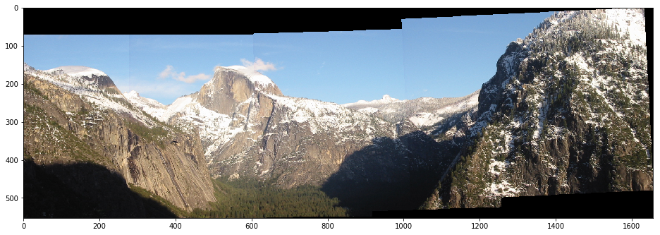
手頃なデータが無かったので、コーネル大学のヨセミテの写真を使いました。
http://www.cs.cornell.edu/courses/cs6670/2011sp/projects/p2/project2.html
大きく間違えてはいないとおもうのですが、結果がパノラマみたいになってしまったのが心残りです。別のデータを使ってまたやってみたいところです。

３章終わり

これで３章終わりです。まだまだ先は長い。