まえおき
先日投稿した「実践コンピュータビジョン」の全演習問題をやってみたの詳細です。なお、あくまで「やってみた」であって、模範解答ではありません。「やってみた」だけなので、うまくいかなかった、という結果もあります。
この記事は「実践コンピュータビジョン」(オライリージャパン、Jan Erik Solem著、相川愛三訳)の演習問題に関する記事です。この記事を書いた人間と書籍との間には何の関係もありません。著者のJan氏と訳者の相川氏にはコンピュータビジョンについて学ぶ機会を与えて頂いたことに感謝します。
実践コンピュータビジョンの原書("Programming Computer Vision with Python")の校正前の原稿は著者のJan Erik Solem氏がCreative Commons Licenseの元で公開されています。。
回答中で使用する画像の多く、また、sfm.py, sift.py, stereo.pyなどの教科書中で作られるファイルはこれらのページからダウンロードできます。
オライリージャパンのサポートページ
Jan Erik Solem氏のホームページ
相川愛三氏のホームページ
ここで扱うプログラムはすべてPython2.7上で動作を確認しています。一部の例外を除きほとんどがJupyter上で開発されました。また必要なライブラリーを適宜インストールしておく必要があります。Jupyter以外の点は、上記の書籍で説明されています。
結構な分量なので章毎に記事をアップしています。今回は第9章です。
9章 画像の領域分割
マイクロソフトリサーチケンブリッジのGrabCutデータ・セットの公開が終了していますが、次のアーカイブからダウンロードすることができました。
https://web.archive.org/web/20161203110733/http://research.microsoft.com/en-us/um/cambridge/projects/visionimagevideoediting/segmentation/grabcut.htm
9.1.1の"build_bayes_graph"がそのままではうまく動作しませんでしたので、以下のように変更しました。
# sigmaのデフォルト値を1e2から1e-2に変更
def build_bayes_graph(im, labels, sigma=1e-2, kappa=2):
    """ Build a graph from 4-neighborhood of pixels.
    Foregraound and background is determined from
    labels (1 for foreground, -1 for background, 0 othewise)
    and is modeled with naive Bayes classifiers. """

    m, n = im.shape[:2]

    vim = im.astype('float')
    vim = vim.reshape((-1, 3))

    foreground = im[labels == 1].reshape((-1, 3))
    background = im[labels == -1].reshape((-1, 3))
    train_data = [foreground, background]

    bc = bayes.BayesClassifier()
    #bc.train(train_data)
    bc.train(train_data, labels) #抜けているlabelsを追加

    bc_lables, prob = bc.classify(vim)
    prob_fg = prob[0]
    prob_bg = prob[1]

    gr = digraph()
    gr.add_nodes(range(m*n+2))

    source = m*n
    sink = m*n+1

    pos = m*n/2-100
    for i in range(vim.shape[0]):
        vim[i] = vim[i] / linalg.norm(vim[i])

    for i in range(m*n):
        gr.add_edge((source, i), wt=(prob_fg[i]/(prob_fg[i] + prob_bg[i])))

        gr.add_edge((i, sink), wt=(prob_bg[i]/(prob_fg[i] + prob_bg[i])))

        if i % n != 0:
            edge_wt = kappa*exp(-1.0*sum((vim[i] - vim[i-1])**2)/sigma)
            gr.add_edge((i, i-1), wt=edge_wt)
        if (i+1) % n != 0:
            edge_wt = kappa*exp(-1.0*sum((vim[i] - vim[i+1])**2)/sigma)
            gr.add_edge((i, i+1), wt=edge_wt)
        if i//n != 0:
            edge_wt = kappa*exp(-1.0*sum((vim[i] - vim[i-n])**2)/sigma)
            gr.add_edge((i, i-n), wt=edge_wt)
        if i//n != m-1:
            edge_wt = kappa*exp(-1.0*sum((vim[i] - vim[i+n])**2)/sigma)
            gr.add_edge((i, i+n), wt=edge_wt)

    return gr
9.4.1 It is possible to speed up computation for the graph cut optimization by reducing the number of edges. This graph construction is described in Section 4.2 of [16]. Try this out and measure the difference graph size and in segmentation time compared to the simpler construction we used.
エッジの数を減らしたグラフカットを文献を参考に試せ
私の回答
文献から、各画素はソースかシンクのどちらか一方にしかリンクをもたない、という方法を試しました。
https://github.com/moizumi99/CVBookExercise/blob/master/Chapter-9/CV%20Book%20Chapter%209%20Exercise%201.ipynb
まずは教科書の方法から。試したのは"empire.jpg"です。
# the original version from Chapter-9
start = time.time()
g = graphcut.build_bayes_graph(im, labels, kappa=1)
res2 = graphcut.cut_graph(g, size)
end = time.time()
print end - start, 's'
411.63883996 s
次に文献の方法
# Reduced version. Each pixel has only one link either to source or to sink
start = time.time()
g = build_bayes_graph(im, labels, kappa=1)
res = graphcut.cut_graph(g, size)
end = time.time()
print end - start, 's'
133.951222181 s
だいぶ速くなりました。肝心の結果は?

だいじょうぶそうですね
9.4.2 Create a user interface or simulate a user selecting regions for graph cut segmentation. Then try "hard coding" background and foreground by setting weights to some large value.
ユーザーに領域を選択させよ
私の回答
自分の使っているJupyter上ではユーザーにインタラクティブに選択させるのは難しそうです。そこは"CV"的には本質でないということで、Jupyter上で座標を表す数値として入力することにします。
https://github.com/moizumi99/CVBookExercise/blob/master/Chapter-9/CV%20Book%20Chapter%209%20Exercise%202.ipynb
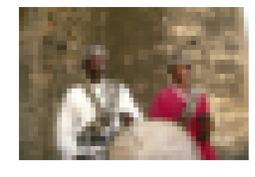
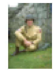
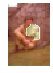
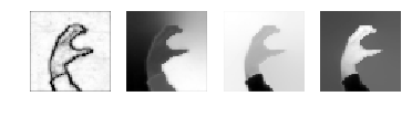
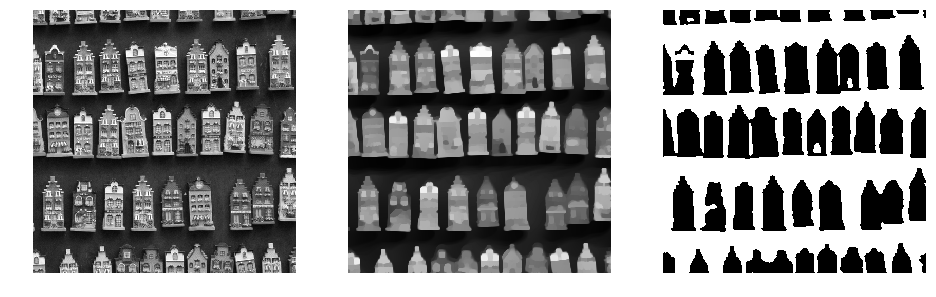
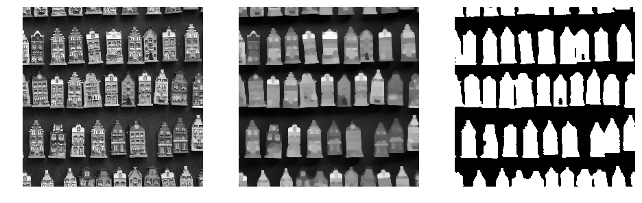
使うのはこの画像です。
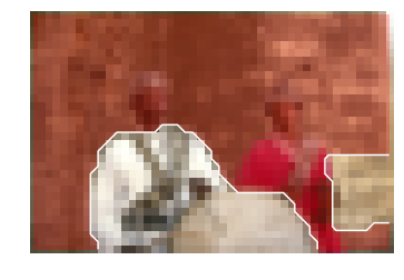
全景と背景を次のようにして指定します
fg = [[16, 24], [32, 32]]
bg = [[0, 0], [48, 8]]
fgが全景、bgが背景です
教科書にならって訓練ラベルを作ります。

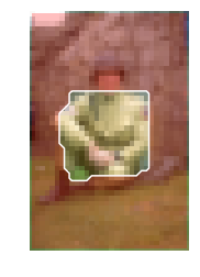
教科書のbays graphの方法を用いて次の結果を得ました。
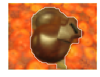
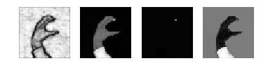
9.4.3 Change the feature vector in the graph cut segmentation from a RGB vector to some other descriptor. Can you improve on the segmentation results?
グラフカットで、特徴量ベクトルをRGBから他の記述子に変更せよ
私の回答
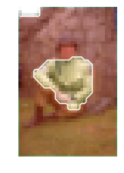
RGBからHSV空間に移してみました。
im2 = colors.rgb_to_hsv(im)
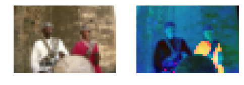
演習問題2と同じ座標を前傾・背景に指定した結果。
こちらの方がいいかもしれません。YUVやLabも気になります。
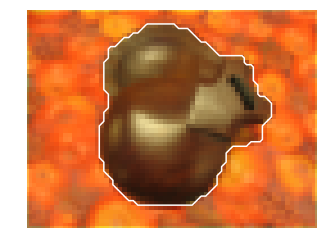
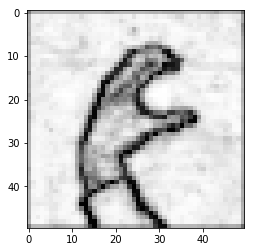
9.4.4 Implement an iterative segmentation approach using graph cut where a current segmentation is used to train new foreground and background models for the next. Does it improve segmentation quality?
繰り返し型の領域分割を実装せよ
私の回答
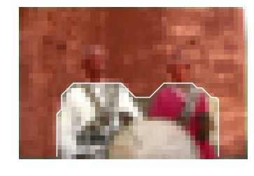
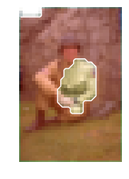
次の図を使います
前景・背景を指定して、一度目の領域分割
その後繰り返しです。
for i in range(4):
    lb = res.copy()
    lb[lb==1] = -1
    lb[lb==0] = 1
    lb[lb==-1] = 0
    lb[:8, :] = -1
    lb[-8:, :] = -1
    lb[:, :2] = -1
    lb[:, -4:] = -1
    g = build_bayes_graph(im, lb, sigma=1e-2, kappa=2, weight=0)
    res = graphcut.cut_graph(g, im.shape[:2])

    figure()
    graphcut.show_labeling(im, res)
    show()

こ、これは、うまくいってませんね。当時のメモにも"This doesn't work."と投げやりなことがかいてあります。失敗です。
9.4.5 The Microsoft Research Grab Cut dataset contains ground truth segmentation maps. Implement a function that measures the segmentation error and evaluate different settings and some of the ideas in the exercises above.
マイクロソフトリサーチのGrab cutデータの正解データを用いて、1-4のアイデアを評価せよ
私の回答

matching score: 0.962565104167

matching score: 0.964518229167
matching score: 0.962890625
matching score: 0.9755859375
意外にもこのデータでは繰り返し法が一番いいけっかでした。繰り返し法は上手くいくときは良い方法のようです。
9.4.6 Try to vary the parameters of the normalized cuts edge weight and see how they affect the eigenvector images and the segmentation result.
エッジ重みパラメータを変えて、固有ベクトルと領域分割にどのような影響があるか調べろ
私の回答
この画像を使います。

パラメータを変えてみましょう
normal_cut(rim, 2, 1e-2)

normal_cut(rim, 0.5, 1e-2)


normal_cut(rim, 1, 2e-2)

normal_cut(rim, 1, 0.5e-2)

normal_cut(rim, 2, 0.5e-2)


最後の図が良さそうです。固有ベクトルの一つが、ほぼ真っ白でひとつだけ点があるのが気になります。
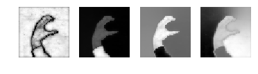
9.4.7 Compute image gradients on the first normalized cuts eigenvectors. Combine these gradient images to detect image contours of objects.
正規化カットの第一固有ベクトルの画像勾配を求め、輪郭を検出せよ
私の回答
第一固有ベクトルはこれになります。
フィルターをかけてみましょう
sigma1 = 1
sigma2 = 3
im2 = filters.gaussian_filter(prime_img, sigma1)
im3 = filters.gaussian_filter(prime_img, sigma2)
im4 = im2 - im3
im5 = sqrt(im4**2)

figure(figsize=(16, 16))
gray()
subplot(3, 2, 1)
imshow(prime_img)
axis('off')
subplot(3, 2, 2)
imshow(im2)
axis('off')
subplot(3, 2, 3)
imshow(im3)
axis('off')
subplot(3, 2, 4)
imshow(im4)
axis('off')
subplot(3, 2, 5)
imshow(im5)
axis('off')
show()
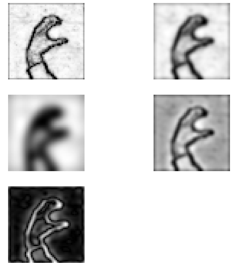
エッジ検出してみます
im6 = im4.copy()
threshold = 0
im6[im6<=threshold] = 0
im6[im6>threshold] = 1
im6 = 1 - im6
figure(0)
gray()
imshow(im6)
axis('off')
show()

9.4.8 Implement a linear search over the threshold value for the de-noised image in Chan-Vese segmentation. For each threshold, store the energy E() and pick the segmentation with the lowest value.
Chan-Vese領域分割の閾値を線形探索せよ
私の回答
次の図の中央の画像から右の画像を作る最適な閾値を探します。
まず、エネルギーを計算する関数を作り、この値が最小になる条件を探します。
def cal_energy(oimg, bimg, lmd):
    imb = bimg.copy()
    imb = 1-imb

    imx = zeros(imb.shape)
    filters.sobel(imb, 1, imx)
    imy = zeros(imb.shape)
    filters.sobel(imb, 0, imy)
    im2 = sqrt(imx**2 + imy**2)

    E_edge = sum(im2)

    imb = 120.0*imb/255 + 40.0/255
    img = 1.0*oimg.copy()/255
    im3 = (img - imb)**2
    E_body = sum(im3)

    return 0.5*lmd*E_edge + E_body, E_edge, E_body

l = 0.5
E_min = 1e10
t_opt = -1
for t in arange(0.2, 0.8, 0.05):
    binimage = 1*(U < t*U.max())
    E, Ee, Eb = cal_energy(im, binimage, l)
    print 't=', t, ': E=', E
    print 'Ee=', Ee, ', Eb=', Eb
    if E<E_min:
        E_min = E
        t_opt = t

t = t_opt
binimage = 1*(U > t*U.max())
print 'best threshold = ', t_opt
t= 0.2 : E= 31137.6292246
Ee= 33940.8393281 , Eb= 22652.4193925
t= 0.25 : E= 27247.6595677
Ee= 57648.4965713 , Eb= 12835.5354248
t= 0.3 : E= 24504.0884836
Ee= 71393.5220391 , Eb= 6655.70797386
t= 0.35 : E= 24413.8613941
Ee= 75370.7802323 , Eb= 5571.16633602
t= 0.4 : E= 24454.2844625
Ee= 77271.4122985 , Eb= 5136.43138793
t= 0.45 : E= 25019.5589919
Ee= 80998.1177979 , Eb= 4770.02954248
t= 0.5 : E= 24891.2522846
Ee= 79578.7336442 , Eb= 4996.56887351
t= 0.55 : E= 25443.4659075
Ee= 78975.6185856 , Eb= 5699.56126105
t= 0.6 : E= 26669.1402989
Ee= 77162.8928527 , Eb= 7378.41708574
t= 0.65 : E= 27085.4658865
Ee= 64899.2706357 , Eb= 10860.6482276
t= 0.7 : E= 26700.0769714
Ee= 45707.3564978 , Eb= 15273.237847
t= 0.75 : E= 26239.0425054
Ee= 28341.2772267 , Eb= 19153.7231988
t= 0.8 : E= 25352.4219484
Ee= 14040.8166823 , Eb= 21842.2177778
best threshold = 0.35
9章終わり
とうとう9章まで終わりました。あと1章です。次はとうとうOpenCVです。いろいろな実用が期待できます