pymcを動かしてみた

環境

mac
python3.5

インストール

pip install pymc

動かしてみる　その１

mymodel.py

# Import relevant modules
import pymc
import numpy as np

# Some data
n = 5 * np.ones(4, dtype=int)
x = np.array([-.86, -.3, -.05, .73])

# Priors on unknown parameters
alpha = pymc.Normal('alpha', mu=0, tau=.01)
beta = pymc.Normal('beta', mu=0, tau=.01)

# Arbitrary deterministic function of parameters
@pymc.deterministic
def theta(a=alpha, b=beta):
    """theta = logit^{-1}(a+b)"""
    return pymc.invlogit(a + b * x)

# Binomial likelihood for data
d = pymc.Binomial('d', n=n, p=theta, value=np.array([0., 1., 3., 5.]),
                  observed=True)

main.py

import pymc
import mymodel

S = pymc.MCMC(mymodel, db='pickle')
S.sample(iter=10000, burn=5000, thin=2)
pymc.Matplot.plot(S)

python main.py

[-----------------65%----              ] 6510 of 10000 complete in 0.5 sec
[-----------------100%-----------------] 10000 of 10000 complete in 0.8 sec
Plotting beta
Plotting alpha
Plotting theta_0
Plotting theta_1
Plotting theta_2
Plotting theta_3

動かしてみる　その２

pip install triangle-plot
pip install corner

jupyter notebook

偽のデータを作成することから始めます。
2つの予測変数（x、y）と1つの結果変数（z）を持つ線形回帰モデルを使用します。

from numpy import *
Nobs = 20
x_true = random.uniform(0,10, size=Nobs)
y_true = random.uniform(-1,1, size=Nobs)
alpha_true = 0.5
beta_x_true = 1.0
beta_y_true = 10.0
eps_true = 0.5
z_true = alpha_true + beta_x_true*x_true + beta_y_true*y_true
z_obs = z_true + random.normal(0, eps_true, size=Nobs)

%matplotlib inline
from matplotlib import pyplot as plt
plt.figure(figsize=(12,6))
plt.subplot(1,2,1)
plt.scatter(x_true, z_obs, c=y_true, marker='o')
plt.colorbar()
plt.xlabel('X')
plt.ylabel('Z')
plt.subplot(1,2,2)
plt.scatter(y_true, z_obs, c=x_true, marker='o')
plt.colorbar()
plt.xlabel('Y')
plt.ylabel('Z')

import pymc
# define the parameters with their associated priors
alpha = pymc.Uniform('alpha', -100,100, value=median(z_obs))
betax = pymc.Uniform('betax', -100,100, value=std(z_obs)/std(x_true))
betay = pymc.Uniform('betay', -100,100, value=std(z_obs)/std(y_true))
eps = pymc.Uniform('eps', 0, 100, value=0.01)

# Now define the model
@pymc.deterministic
def model(alpha=alpha, betax=betax, betay=betay, x=x_true, y=y_true):
    return alpha + betax*x + betay*y

# pymc parametrizes the width of the normal distribution by tau=1/sigma**2
@pymc.deterministic
def tau(eps=eps):
    return power(eps, -2)

# Lastly relate the model/parameters to the data
data = pymc.Normal('data', mu=model, tau=tau, value=z_obs, observed=True)

定義が整ったらpymc.MCMCにpymcオブジェクトを送り、サンプラーを作成して実行します。
ここではuse_step_methodを使用してMetropolis-Hastingsサンプラーを適応しています。
これはデフォルトMetropolis-Hastingsよりも賢いサンプラーです。
より効率的にパラメータ空間をサンプリングするために、以前のサンプルを使用して共分散行列を構築します。

sampler = pymc.MCMC([alpha,betax,betay,eps,model,tau,z_obs,x_true,y_true])
sampler.use_step_method(pymc.AdaptiveMetropolis, [alpha,betax,betay,eps],
                        scales={alpha:0.1, betax:0.1, betay:1.0, eps:0.1})
sampler.sample(iter=10000)

[100%**] 10000 of 10000 complete

プロットします。

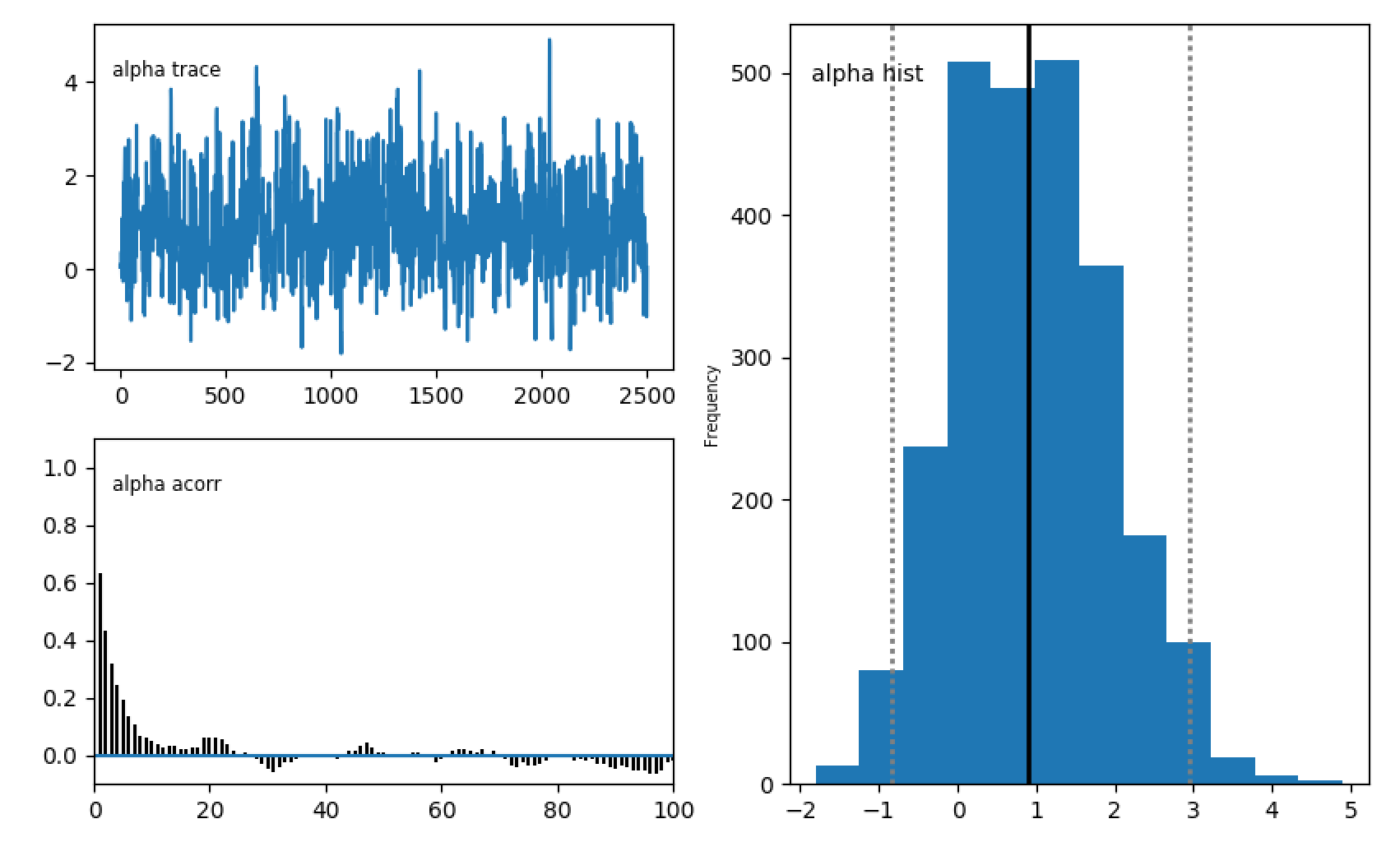
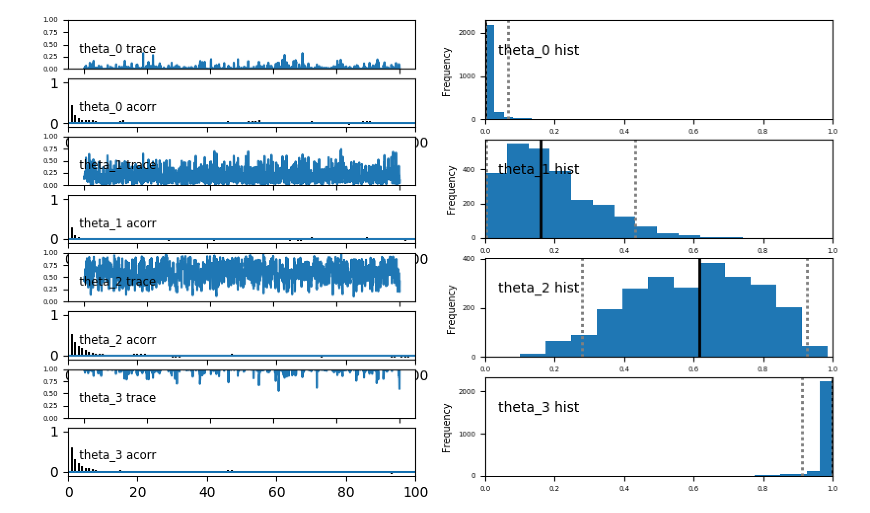
pymc.Matplot.plot(sampler)

アルファだけ貼り付けておきます。
それぞれの確率について、pymcはトレース（左上のパネル）、自己相関（左下のペイン）、およびサンプルのヒストグラム（右のパネル）をプロットします。 最初はあまり何も起こらないことがわかります。その後、適応MHサンプラーはより良い共分散行列を見つけるようになります。

次は各変数の中央値をサンプルから取得しましょう。
MCMCサンプルでは、​​各変数のトレースを調べます。

m_alpha = median(alpha.trace())
m_betax = median(betax.trace())
m_betay = median(betay.trace())
m_eps = median(eps.trace())

中央値は、非対称分布（例えば、epsの分布）に対してより頑強である。
今回はプロットとxを逆にするときのy予測子を修正します。
そうすれば、正しいトレンドが見つかったかどうかを確認できます。
本質的なばらつきを表す影付き領域をプロットすることもできます。

plt.figure(figsize=(12,6))
plt.subplot(1,2,1)
plt.plot(x_true, z_obs-m_alpha-m_betay*y_true, 'o')
plt.xlabel('X')
plt.ylabel('Z - alpha - beta_y y')
# Now plot the model
xx = array([x_true.min(), x_true.max()])
plt.plot(xx, xx*m_betax)
plt.plot(xx, xx*m_betax + m_eps, '--', color='k')
plt.plot(xx, xx*m_betax - m_eps, '--', color='k')
plt.subplot(1,2,2)
plt.plot(y_true, z_obs-m_alpha-m_betax*x_true, 'o')
plt.xlabel('Y')
plt.ylabel('Z - alpha - beta_x x')
yy = array([y_true.min(), y_true.max()])
plt.plot(yy, yy*m_betay)
plt.plot(yy, yy*m_betay + m_eps, '--', color='k')
plt.plot(yy, yy*m_betay - m_eps, '--', color='k')

triangle_plotプロットパッケージで、さまざまなパラメータの共分散を調べる。
これを行うには、[i、p]でインデックス付けされた2次元配列のマルコフ連鎖が必要らしい。
全要素をsamplesに連結して転置する。

samples = array([alpha.trace(),betax.trace(),betay.trace(),eps.trace()]).T
print((samples.shape))
import triangle
triangle.corner(samples[:,:], labels=['alpha','betax','betay','eps'], truths=[alpha_true, beta_x_true, beta_y_true, eps_true])

使用例

参考

https://users.obs.carnegiescience.edu/cburns/ipynbs/PyMC.html
https://pymc-devs.github.io/pymc/INSTALL.html#dependencies