WaveNetの確率分布を観察することで,何か研究に活かせるのではと思い,こちらの実装を動かしてみた.しかし,出力のTensorのデータ構造がMoLのどのパラメータなのか理解できずに苦労したため,そのメモを記す
参考リンク
- An Explanation of Discretized Logistic Mixture Likelihood
- Doubt on use of discretized MoL in sampling and loss calclation
ロジスティック分布
こちらのサイトを参考に,ロジスティック分布は,以下の式で表される連続確率分布である.
p(x;\mu,s) = \frac{\exp(-\frac{x-\mu}{s})}{s(1+\exp(-\frac{x-\mu}{s}))^2}
また,分布は以下の様になる.
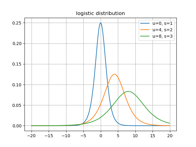
分布の形状は正規分布とよく似ているが,ロジスティック分布のほうが裾が広いため,平均から離れた値でも確率が0になりにくいとのこと.
混合ロジスティック分布(Mixture of Logistic)
確率分布の混合モデルは,係数倍したそれぞれの確率分布の和で表される.
p(x) = \sum^{K}_{i=1}\pi_i logistic(\mu _i,s_i)
ここでは係数を$\pi$,ロジスティック分布の確率密度関数を$logistic(\mu, s)$とする.また,例として先程の分布をすべて係数1で足し合わせた混合モデルを以下に記す.
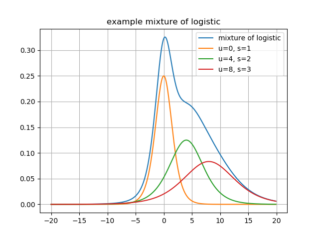
基本的に,この確率分布からサンプリングを行うことで出力を得るのが一般的である.
引っかかってしまった点
動かした実装から,サンプリングを行っている箇所を引用すると
# sample mixture indicator from softmax
temp = logit_probs.data.new(logit_probs.size()).uniform_(1e-5, 1.0 - 1e-5)
 temp = logit_probs.data - torch.log(- torch.log(temp))
 _, argmax = temp.max(dim=-1)
# (B, T) -> (B, T, nr_mix)
 one_hot = to_one_hot(argmax, nr_mix)
 # select logistic parameters
 means = torch.sum(y[:, :, nr_mix:2 * nr_mix] * one_hot, dim=-1)
 log_scales = torch.sum(y[:, :, 2 * nr_mix:3 * nr_mix] * one_hot, dim=-1)
 if clamp_log_scale:
     log_scales = torch.clamp(log_scales, min=log_scale_min)
 # sample from logistic & clip to interval
 # we don't actually round to the nearest 8bit value when sampling
 u = means.data.new(means.size()).uniform_(1e-5, 1.0 - 1e-5)
 x = means + torch.exp(log_scales) * (torch.log(u) - torch.log(1. - u))
x = torch.clamp(torch.clamp(x, min=-1.), max=1.)
となっている.しかし,混合分布を計算する箇所がなく,どのように確率分布を求めてサンプリングしているのかがわからなかった.そこで調べた所,Gumbel-max trickとinversion samplingというテクニックを使っていた.

## Gumbel-max trick
Gumbel-max trickは[Doubt on use of discretized MoL in sampling and loss calclation](https://github.com/Rayhane-mamah/Tacotron-2/issues/155)でこのように述べられている.

>It turns out there is something called Gumbel-max trick which mimics a softmax sampling. So basically, the idea here is that we apply a softmax-like sampling to select which Logistic distribution to use.

つまり,混合分布を計算してサンプリングを行うのではなく,どのパラメータのロジスティック分布を用いるかを`logit_prob`というカテゴリカル分布からのサンプリングで決定している,ということである.
### なぜこのようなサンプリングをするか
これに関して調べたところ,[Categorical Reparameterization with Gumbel-Softmax](https://arxiv.org/abs/1611.01144)という論文を発見,[こちらのサイト](http://musyoku.github.io/2016/11/12/Categorical-Reparameterization-with-Gumbel-Softmax/)の解説を引用すると

>カテゴリカル分布からのサンプリングは一般的に、データxとパラメータ$\phi$のニューラルネット$f_\phi$、さらにsoftmax関数を用いて

>```math
z\sim softmax(f_\phi(x))
のように行います。
(クラス分類の場合はサンプリングではなくargmaxで確率最大のクラスを取ります)
得られたサンプルzはパラメータ$\phi$で微分することができないため、この論文ではGumbel-Softmax分布を用いたreparameterization trickにより微分可能なサンプリングを実現しています。
とのこと.このサンプリングであるメリットというより,学習の都合上このようなテクニックを使っている,ということが考えられる.このあたりに関しては,もう少しPixel CNN++の論文を読む等調査が必要である.
inversion sampling
inversion sampling,日本語では逆関数法と呼ばれる乱数生成のテクニック.逆関数法を用いた乱数生成の証明と例から引用すると
逆関数法:累積分布関数が $F(x)$ であるような確率分布に従う乱数を生成したいときには,
[0,1] 上の一様分布に従う乱数を生成してそれに $F^{−1}$ をかませばよい。
このことから,生成する乱数自体が,目的のロジスティック分布の累積分布関数に従うように設計されている.
メリット
Doubt on use of discretized MoL in sampling and loss calclationから引用すると
Now to sampling, for MoL, we use something called inversion sampling. I always see people asking why we switch to CDF (sigmoid) when using Logistic distribution, it actually makes training and sampling from the distribution very easy. Let's first consider the CDF of the Logistic distribution equation (1):
y = \frac{1}{1 + e^{-\frac{(x - \mu)}{s}}}
>The main idea of sampling is that we want to pick a random variable X that is most probable to be picked using the Distribution $L(\mu, s)$ . The idea of inverse sampling is to do that but using the CDF formula. i.e: we want to pick a random variable X that is most probable under the Logistic PDF. By doing some simple calculation we can indeed find the equation (quantile function (2)):

>```math
X = \mu + s\ \log(\frac{y}{1 - y})
In practice, we select a random uniform y in (1e-5, 1 - 1e-5) to avoid saturation regions of the sigmoid, then determine x from it. If things got a bit too complicated at this point, use Logistic distribution link above for plot assistance. Naturally, it is evident to notice that if our randomly picked y=0.5, x will be exactly the mean of the Logistic distribution, which is logic. Lucky for us, by picking a y between 1e-5 and 1 - 1e-5 we can actually get a x that is most probable for those mean and scale parameters according to PDF.
ロジスティック分布の累積分布関数はsigmoid関数と同じである.これにより,分布の学習とサンプリングが簡単になるため行っていると記述がある.また,sigmoid関数を使うため,1e-5から1-1e-5の一様分布から乱数を生成することで飽和を起こさないようにしている.
なぜロジスティック分布を使うか
一般的に,確率モデルではガウス分布が用いられることが多いが,なぜロジスティック分布なのかと疑問に思っていた.今回inversion samplingを調べていて思ったことであるが,ロジスティック分布は正規分布と比べて累積分布関数を簡単に求めることができる.inversion samplingを用いることで学習,サンプリングを簡単にすることができる,といった理由と合わせて考えると正規分布の混合分布でモデリングを行わなかったのではないかと考察している.正規分布の累積分布関数はこちら
調べて思ったこと
論文における数学的な話と,計算機で実行する上での効率の良いアルゴリズムという双方の理解が必要なので中々大変だなと感じた.しかし,混合分布からサンプリングを効率よく行う方法を知ることができたため,今後深層生成モデルを検討する際には活用していきたい.
まとめ
- MoLからサンプリングを行う際,Gumbel-max trickとinversion samplingというテクニックを使う
- 混合分布を直接計算するのではなく,Gumbel-max trickを用いてサンプリングを行うロジスティック分布のパラメータを決定する
- inversion samplingを用いて,ロジスティック分布からのサンプリングを簡単にしている
今後は,どのようにlogit_probやロジスティック分布のパラメータを学習しているかもしっかり理解していきたいと考えている.