この記事について
この記事では最適制御の簡単な例題として, 単振動の制御を行います. シミュレーションはpython (numpy, scipy)で行います. また, 最適制御をよく理解するために, 線形フィードバック制御との比較も行います.
なお, この記事では, 具体的な計算方法を示すことを目的としているため, 変分法などによる計算式の導出は割愛しております. ご興味のある方は, 参考文献や他の記事などを参照してください.
問題設定: 運動方程式と制御関数

今回の問題設定を上図に示します. 外力$u(t)$を加えることで, 単振動の動きを止めることが目標です. このシステム全体の運動方程式は, 質量を$m$, ばね係数を$k$とすると, 以下のようになります:
m\ddot{x}= -kx + u.
今回は簡単のため、$m=1, k=1$とします:
\ddot{x} = -x + u.
まず, 上式を連立常微分方程式の形式に変形します:
\begin{align}
\dot{x} &= v \\
\dot{v} &= -x + u.
\end{align}
さらにベクトル $y=(x,v)^T$を用いることで, 以下のようにまとめることができます:
$$ \dot{y} = Ay + Bu,$$
A=\left(
\begin{matrix}
0 & 1 \\
-1 & 0
\end{matrix}
\right), ~B=\left(
\begin{matrix}
0  \\
1
\end{matrix}
\right).
今回, 最小化したい関数(コスト関数)は
J=\frac{1}{2}\int _{t_i} ^{t_f} (x^2 + \gamma u^2) dt
とします. ここで, $t_i$は開始時刻, $t_f$は終了時刻を表します. また, 加える力$u(t)$の大きさにペナルティを与えており, $\gamma$の値が大きいほど, より小さい力で制御をすることが求められます. 結局, このコスト関数の最小化の意味するところは, ``より小さい力で制御しつつ, 質点の位置をより早く0へ収束させる'' となります。
上式を, 慣習に倣い二次形式に変形すると,
J=\frac{1}{2}\int _{t_i} ^{t_f} (y^TQy + u^TRu)dt \\
Q=\left(
\begin{matrix}
1 & 0 \\
0 & 0
\end{matrix}
\right),~ R=\gamma,
となります. それでは, 以降で線形フィードバック, 及び最適制御によって, コスト関数の最小化を目指します.
線形フィードバックによる制御
この問題は、制御システムが線形, コスト関数が二次形式のLQ制御問題であり, 最適レギュレーター理論から, 制御関数が以下のように得られます:
u=-R^{-1}B^TSy.
ここで$S$は2x2の行列でありリッカチ方程式:
A^TS + SA - SBR^{-1}B^TS + Q = 0
の解です. これは固有値分解により効率的に解くことができ, scipyでソルバー(scipy.linalg.solve_continuous_are)が提供されています. 様々な$\gamma$の値 (0.1, 1, 10) のときのシミュレーションの結果を下図に示します.
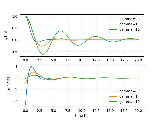
$\gamma$の値が小さいときは($\gamma=0.1$), 値が大きいとき($\gamma=10$)のときよりも位置$x$の収束が早いことがわかります. これは, より大きなフィードバック$u$を用いているためです.
非線形最適制御
それでは, 本題の非線形制御に移ります. 非線形制御では, 先に用いたような線形フィードバック ($u=My$) のような仮定をおかず, 最適な制御関数$u^*(t)$を直接求めます. なお, 以降では, $\gamma = 1$の場合について考えます.
問題の定式化
運動方程式をもう一度書き記します:
$$ \dot{y} = Ay + Bu=f(y,u). $$
最適制御では, 以下のようにコスト関数を定義します.
\bar{J}= \int _{t_i} ^{t_f} \left(\frac{x^2 + \gamma u^2}{2} + \lambda^T(f-\dot{y})\right) dt
ここで$\lambda$はアジョイント(ラグランジュ乗数)と呼ばれる関数です. さらに, 最適制御理論におけるハミルトニアン$H$を便宜的に定義します:
H(y,u,\lambda)=\left(\frac{x^2 + \gamma u^2}{2} + \lambda^Tf\right).
さて, 最適な制御$u(t)=u^*(t)$が存在する場合, コスト関数 ($\bar{J}$) の変数 ($y, \dot{y}, u, \lambda$) に対する変分が0となる条件から, 以下の条件が導出されます:
\dot{\lambda}=-\left( \frac{\partial H}{\partial y} \right)^T, ~\lambda(t_f)=0, ~\frac{\partial H}{\partial u}=0.
これらを具体的に書き記すと以下のようになります:
\begin{align}
\dot{\lambda}&=-\left( \frac{\partial H}{\partial y} \right)^T
=-\left(
\begin{matrix}
\frac{\partial H}{\partial x} \\
\frac{\partial H}{\partial v}
\end{matrix}
\right)=-\left(
\begin{matrix}
x+\lambda^TA\left(\begin{matrix}
1\\
0
\end{matrix}\right)
 \\
\lambda^TA\left(\begin{matrix}
0\\
1
\end{matrix}\right)
\end{matrix}
\right),
\end{align}
\frac{\partial H}{\partial u}=\gamma u+\lambda ^TB=0.
アジョイント($\lambda$)の微分方程式は終端 ($t=t_f$) での値が決められているので, 微分方程式を逆時間方向に (過去に遡って) 解くことで計算することができます. アジョイントとハミルトニアンの微分$\frac{\partial H}{\partial u}$を, さきほどの線形フィードバック制御関数$u(t)$を用いて, 計算しました.
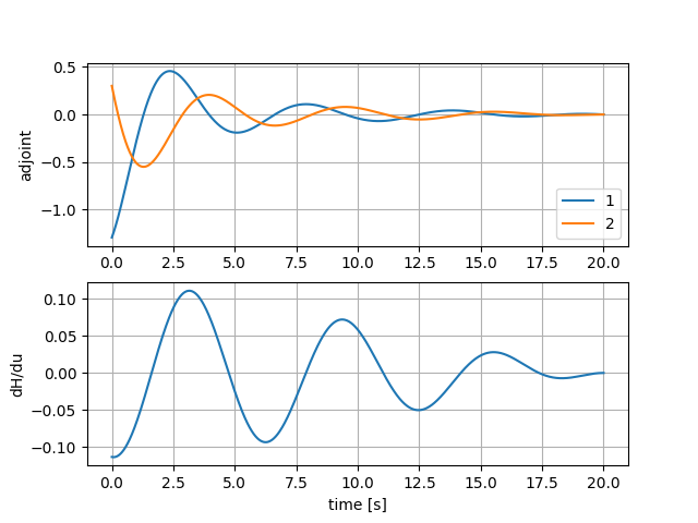
下段の$\frac{\partial H}{\partial u}$の時間発展をみると, 明らかに最適性の条件$\frac{\partial H}{\partial u}=0$を満たしていないことがわかります. つまり, 線形フィードバック制御により計算された$u(t)$は最適でないことがわかります.
勾配法による最適化
線形フィードバックにより得られた制御関数$u(t)$は, コスト関数の停留条件 $\left(\frac{\partial H}{\partial u}=0\right)$ を満たさないので, 最適でないことがわかりました. そこで, 今度は直接, コスト関数を最小化することを考えます:
\min _u \left(\bar{J}\right).
最小化する方法はいくつかありますが, 今回は最も一般的な勾配法を用います. 勾配法は, 制御関数を
u^\text{new}(t) = u^\text{old}(t) + \eta \delta u(t)
のように繰り返し更新することでコスト関数を最小化します. ここで, $\delta u$は, コスト関数が減少する方向であり, $\eta >0$は, 更新の大きさを決める定数です. 変分法により, コスト関数の変分がゼロでない部分は,
\delta \bar{J} = \int _{t_i} ^{t_f} \frac{\partial H}{\partial u}\delta u~dt
と示すことができるため,
\delta u = -\left(\frac{\partial H}{\partial u}\right)^T,
とおくと, $\delta \bar{J}<0$となり, 制御関数$u(t)$の更新によりコスト関数を小さくすることができます. つまり, 以下のように更新を繰り返します:
u^\text{new}=u-\eta \cdot \left(\frac{\partial H}{\partial u}\right)^T.
$\eta$の値は, 一般的には直線探索法によって決定できますが, 今回は, よりシンプルな方法として, 固定した値 $(\eta =0.004)$で更新を繰り返しました. また, $u(t)$の初期条件として, 線形フィードバックから得られたものを用いました. 結果を以下の図に示します.
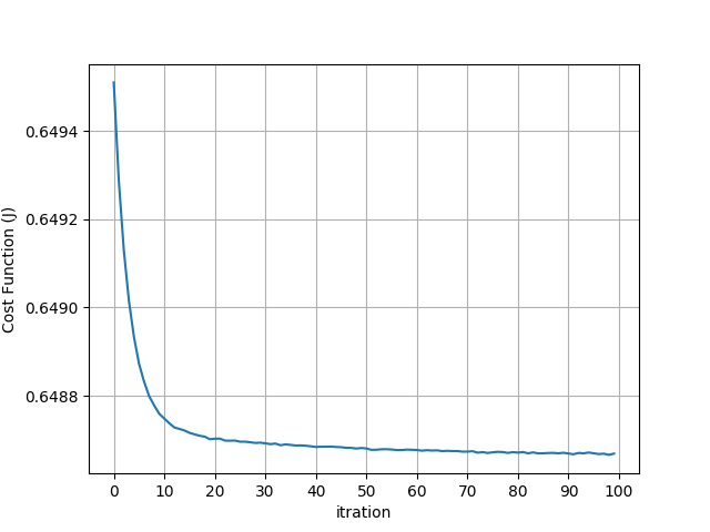
更新毎にエラー($J$)が減少していき, 100回程度で収束しました. 次に, 最適化前と最適化後の質点の動きと, 制御関数の変化, および, ハミルトニアンの微分を以下の図に示します.
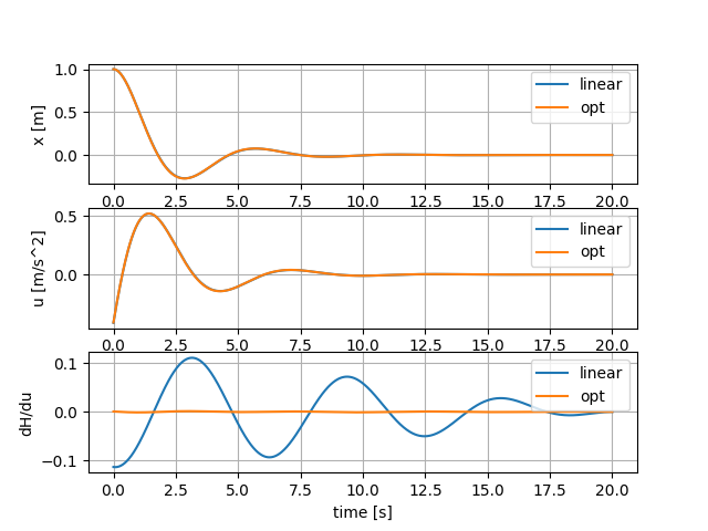
まず, 下段についてですが, 最適化された場合は(opt), 最適化の条件$\frac{\partial H}{\partial u}=0$をほぼ満たています. しかし, 質点の動き $(x)$ はほとんど変化がなく, 下図のように拡大すると何とかわかる程度です.
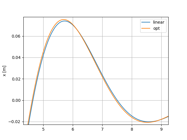
これは, 線形フィードバックが元々最適解にかなり近かったことを示しています.
まとめ
線形システムである単振動に対して, 最適制御と線形フィードバック制御との比較をおこないました. 制御対象が線形なため, 二つの制御の結果に大きな違いは得られませんでしたが, 確かに, 最適制御は線形制御よりもコスト関数を小さくすることがわかりました.
コード
作成したコードを公開します. 線形フィードバック制御のコードはriccati.pyです. 非線形制御については, 運動方程式等はsystem.pyで記述されており, main.pyが勾配法により制御関数を更新するために, system.pyをループ計算します. plot_opt.pyは計算結果を表示します.
riccati.py: 線形フィードバック制御のコード
  1 import numpy as np
  2 import scipy as sp
  3 from scipy import linalg
  4 from scipy import integrate
  5
  6 def calc_u(y, B, S):
  7   return -1./R * np.dot(B.transpose(), np.dot(S,y))
  8
  9 def func(y, t, A, B,R,S):
 10   # u = -1./R * np.dot(B.transpose(), np.dot(S,y))
 11   u = calc_u(y, B, S)
 12   dydt = np.dot(A,y) + np.dot(B,u)
 13   return dydt
 14
 15 gamma = 10 # regularization coefficient
 16 t_0 = 0 # initial time
 17 t_f = 20 # final time
 18 t_n = 1000 # number of memory
 19 y0 = np.array([1,0]) # Initial condition
 20
 21 t = np.linspace(t_0, t_f, t_n)
 22
 23 A = np.array([[0,1], [-1,0]])
 24 B = np.array([[0],[1]])
 25 Q = np.array([[1,0],[0,0]])
 26 R = gamma
 27
 28 print("Solving Riccati equation...")
 29 S = sp.linalg.solve_continuous_are(A,B,Q, R)
 30
 31 print("Solving ODE...")
 32 y = sp.integrate.odeint(func, y0, t, args=(A,B,R,S))
 33 print("Calculating u...")
 34 u = np.zeros(len(t))
 35 for i in range(len(t)):
 36   u[i] = calc_u(y[i], B, S)
 37
 38 def y_approx(t, y, t_f, t_n):
 39   t_index = (t_n-1)*(t/t_f)
 40   #t_index = t_index.astype(int)
 41   t_index = int(t_index)
 42   return y[t_index]
 43
 44
 45 # ===== Save Data =====
 46 print("Saving y and u...")
 47
 48 np.savetxt("./data/y_gamma_{0}.dat".format(gamma), y, delimiter=",")
 49 np.savetxt("./data/u_gamma_{0}.dat".format(gamma), u, delimiter=",")
 50
system.py: 非線形制御の計算(運動方程式, アジョイント, etc.)
  1 import numpy as np
  2 import scipy as sp
  3 from scipy import linalg
  4 from scipy import integrate
  5
  6 import matplotlib.pyplot as plt
  7
  8
  9 def func(y, t, A, B, u, t_f, t_n):
 10   dydt = np.dot(A,y) + np.dot(B,u_approx(t, u, t_f, t_n)).reshape(2)
 11   return dydt
 12
 13 def y_approx(t, y, t_f, t_n):
 14     t_index = (t_n-1)*(t/t_f)
 15     t_index = int(t_index)
 16     t_index = min([t_index, 999])
 17     return y[t_index]
 18
 19 def u_approx(t, u, t_f, t_n):
 20   t_index = (t_n-1)*(t/t_f)
 21   t_index = int(t_index)
 22   t_index = min([t_index, 999])
 23   return u[t_index]
 24
 25 def f_adjoint_inv(adjoint, t, y, A, t_f, t_n):
 26     deriv1 =  y_approx(t, y, t_f, t_n)[0] + np.dot(adjoint.transpose(), n    p.dot(A, np.array([[1],[0]])))
 27     deriv2 =  np.dot(adjoint.transpose(), np.dot(A, np.array([[0],[1]])))
 28     deriv = np.array([deriv1,deriv2])
 29     deriv = deriv.reshape(2)
 30     return deriv
 31
 32 def J_integrand(y_this, t, y, u, t_f, t_n, gamma):
 33   x = y_approx(t, y, t_f, t_n)[0]
 34   u = u_approx(t, u, t_f, t_n)
 35   dydt = (x*x + gamma*u*u)/2.
 36   return dydt
 37
 38 def system(u, t_0, t_f, t_n, gamma):
 39
 40   # ===== Hyper parameters =====
 41   y0 = np.array([1,0]) # Initial condition
 42
 43   # ===== Matrices for motion =====
 44   t     = np.linspace(t_0, t_f, t_n)
 45   t_inv = np.linspace(t_f, t_0, t_n)
 46   A = np.array([[0,1],[-1,0]])
 47   B = np.array([[0],[1]])
 48   Q = np.array([[1,0],[0,0]])
 49   R = gamma
 50
 51   print("Solving ODE...")
 52   y = sp.integrate.odeint(func, y0, t, args=(A,B,u, t_f, t_n))
 53
 54   # ===== Solve Adjoint Problem =====
 55   print("Solving adjoint...")
 56   adjoint = sp.integrate.odeint(f_adjoint_inv, np.array([0,0]), t_inv, ar    gs=(y, A, t_f, t_n))
 57
 58   # correct the time order
 59   adjoint = np.flipud(adjoint)
 60   H_u = gamma * u + np.dot(adjoint, B).transpose()
 61   H_u = H_u.transpose()
 62
 63   print("Calculate Loss")
 64
 65   J = sp.integrate.odeint(J_integrand, 0, t, args=(y, u, t_f, t_n, gamma)    )
 66
 67   return y, adjoint, H_u, J[-1]
 68
 69
 70 if __name__ == "__main__":
 71
 72
 73   gamma = 1 # regularization coefficient
 74
 75
 76   u = np.loadtxt("./data/u_gamma_{0}.dat".format(gamma), delimiter=",")
 77   t_0 = 0 # initial time
 78   t_f = 20 # final time
 79   t_n = 1000 # number of memory
 80
 81   y, adjoint, H_u, J = system(u, t_0, t_f, t_n, gamma)
 82
 83   t = np.linspace(t_0, t_f, t_n)
 84
 85   # ===== Plot results =====
 86
 87   plt.subplot(3,1,1)
 88   plt.plot(t, y[:,0], label="x")
 89   plt.legend()
 90
 91   plt.subplot(3,1,2)
 92   plt.plot(t, y[:,1], label="v")
 93   plt.legend()
 94
 95   plt.subplot(3,1,3)
 96   plt.plot(t, u, label="u")
 97   plt.legend()
 98   plt.show()
 99
100   plt.subplot(3,1,1)
101   plt.plot(t, u, label="u")
102   plt.legend()
103   plt.grid()
main.py: 勾配法で制御関数を更新します.
  1 import numpy as np
  2 import scipy as sp
  3 from scipy import linalg
  4 from scipy import integrate
  5
  6 import matplotlib.pyplot as plt
  7
  8 import system
  9
 10 # ===== Hyper parameters =====
 11 gamma = 1 # regularization coefficient
 12 t_0 = 0. # initial time
 13 t_f = 20. # final time
 14 t_n = 1000. # number of memory
 15 y0 = np.array([1,0]) # Initial condition
 16
 17 u = np.loadtxt("./data/u_gamma_{0}.dat".format(gamma), delimiter=",")
 18
 19 t_0 = 0 # initial time
 20 t_f = 20 # final time
 21 t_n = 1000 # number of memory
 22
 23 # === Gradient Descent Parameters ===
 24 itr = 100
 25 eta = 0.004 # learning rate
 26
 27 J = np.zeros(itr)
 28
 29 for i in range(itr):
 30   print("itr: {0}".format(i))
 31   y, adjoint, H_u, J[i] = system.system(u, t_0, t_f, t_n, gamma)
 32   print("Error: {0}".format(J[i]))
 33   if (i==0):
 34     print("Saving files for linear feedback case..")
 35     np.savetxt("./data/adjoint_gamma_{0}.dat".format(gamma), adjoint, del    imiter=",")
 36     np.savetxt("./data/H_u_gamma_{0}.dat".format(gamma), H_u, delimiter="    ,")
 37   u = u - eta * H_u.reshape(1000) # why error happens???
 38
 39
 40 t = np.linspace(t_0, t_f, t_n)
 41
 42 np.savetxt("./data/y_opt_gamma_{0}.dat".format(gamma), y, delimiter=",")
 43 np.savetxt("./data/u_opt_gamma_{0}.dat".format(gamma), u, delimiter=",")
 44 np.savetxt("./data/H_u_opt_gamma_{0}.dat".format(gamma), H_u, delimiter="    ,")
 45 np.savetxt("./data/J_gamma_{0}.dat".format(gamma), J, delimiter=",")
 46
 47 plt.plot(J)
 48 plt.grid()
 49 plt.legend()
 50 plt.show()
plot_opt.py: 結果の表示
  1 import numpy as np
  2 import matplotlib.pyplot as plt
  3
  4 gamma = 1
  5
  6 t = np.linspace(0,20, 1000)
  7 y    = np.loadtxt("./data/y_gamma_{0}.dat".format(gamma), delimiter=",")
  8 y_opt   = np.loadtxt("./data/y_opt_gamma_{0}.dat".format(gamma), delimite
    r=",")
  9 u    = np.loadtxt("./data/u_gamma_{0}.dat".format(gamma), delimiter=",")
 10 u_opt  = np.loadtxt("./data/u_opt_gamma_{0}.dat".format(gamma), delimiter
    =",")
 11 H_u  = np.loadtxt("./data/H_u_gamma_{0}.dat".format(gamma), delimiter=","
    )
 12 H_u_opt  = np.loadtxt("./data/H_u_opt_gamma_{0}.dat".format(gamma), delim
    iter=",")
 13
 14 plt.subplot(3,1,1)
 15 plt.plot(t, y[:,0], label="linear")
 16 plt.plot(t, y_opt[:,0], label="opt")
 17 plt.legend()
 18 plt.grid()
 19 plt.ylabel("x [m]")
 20
 21 plt.subplot(3,1,2)
 22 plt.plot(t, u, label="linear")
 23 plt.plot(t, u_opt, label="opt")
 24 plt.legend()
 25 plt.grid()
 26 plt.xlabel("time [s]")
 27 plt.ylabel("u [m/s^2]")
 28
 29 plt.subplot(3,1,3)
 30 plt.plot(t, H_u, label="linear")
 31 plt.plot(t, H_u_opt, label="opt")
 32 plt.legend()
 33 plt.grid()
 34 plt.xlabel("time [s]")
 35 plt.ylabel("dH/du")
 36 plt.show()
参考文献
・「非線形最適制御理論入門」, 大塚 敏之 (2011)